Tutorial - Building a QGAN to Generate a Two-Qubit State Using Pennylane and Tensorflow
Generative adversarial networks (GANs) are fundamentally composed of two "characters" - a generator and a discriminator. By putting these two buddies "to war", we will result in an outcome when the data that the generator generates becomes equal to the real data, even though the generator is never told what the real data is. That's essentially the purpose of a GAN - to generate data that mimics some sort of real data, whether it's generating pictures of people that mimics real pictures or generating counterfeit bills that mimic real bills. This blog post will focus on the technical implementation details of a quantum GAN (QGAN) that can generate a 2-qubit state. If you're looking to build a theoretical understanding, I recommend this video.
In a classical GAN, the generator and discriminator are created as neural networks. In a quantum GAN, the generator and discriminator are created as quantum neural networks (QNNs), or, parametized quantum circuits (PQCs). (These two terms refer to the same thing.)

Image source: @EliesMiquel on Twitter
Note: If the images are not showing up, try viewing the notebook via this link.
We start off with our imports:
import pennylane as qml
import tensorflow as tf
from pennylane import numpy as np
from matplotlib import pyplot as plt
INFO:tensorflow:Enabling eager execution
INFO:tensorflow:Enabling v2 tensorshape
INFO:tensorflow:Enabling resource variables
INFO:tensorflow:Enabling tensor equality
INFO:tensorflow:Enabling control flow v2
Quantum Circuit Architecture
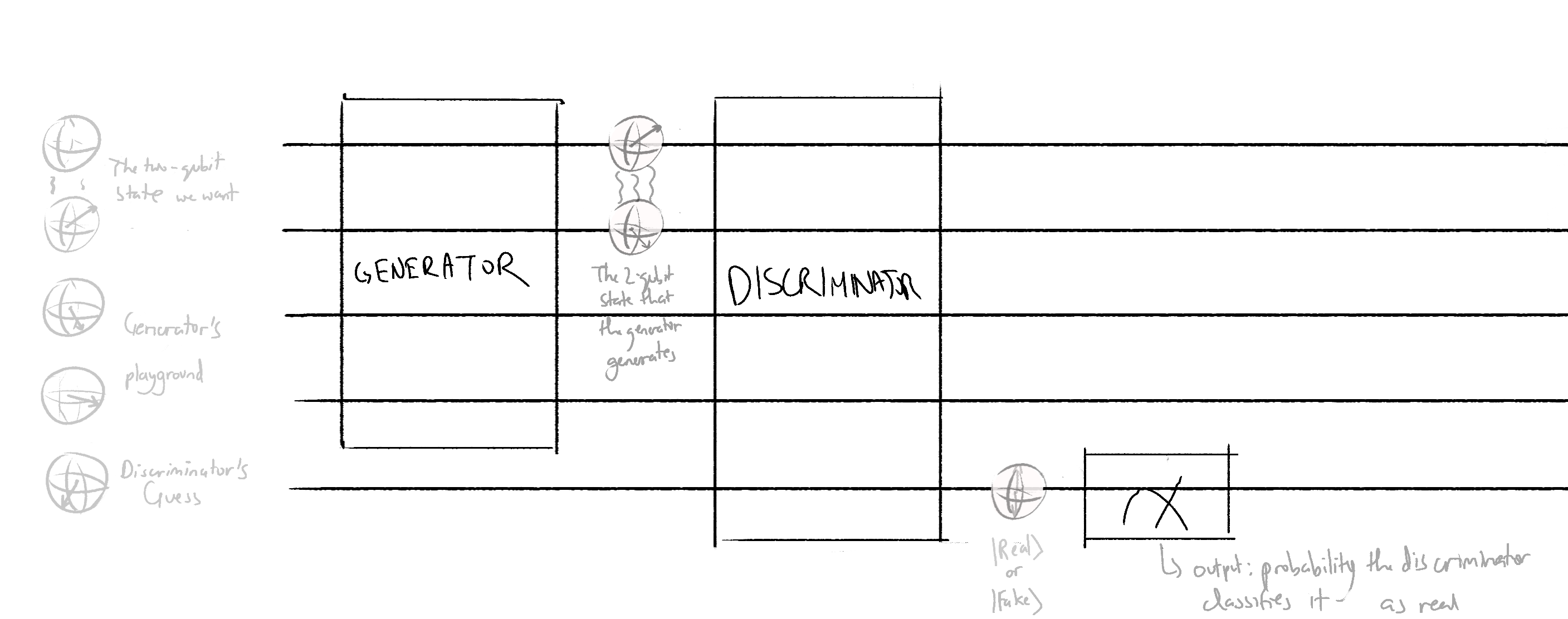
I used 5 qubits:
- Qubit 0 & 1: the 2 qubit state that we are trying to generate
- Qubit 2 & 3: the generator's playground
- Qubit 4: the generator's guess
num_wires = 5

dev = qml.device('cirq.simulator', wires=num_wires)
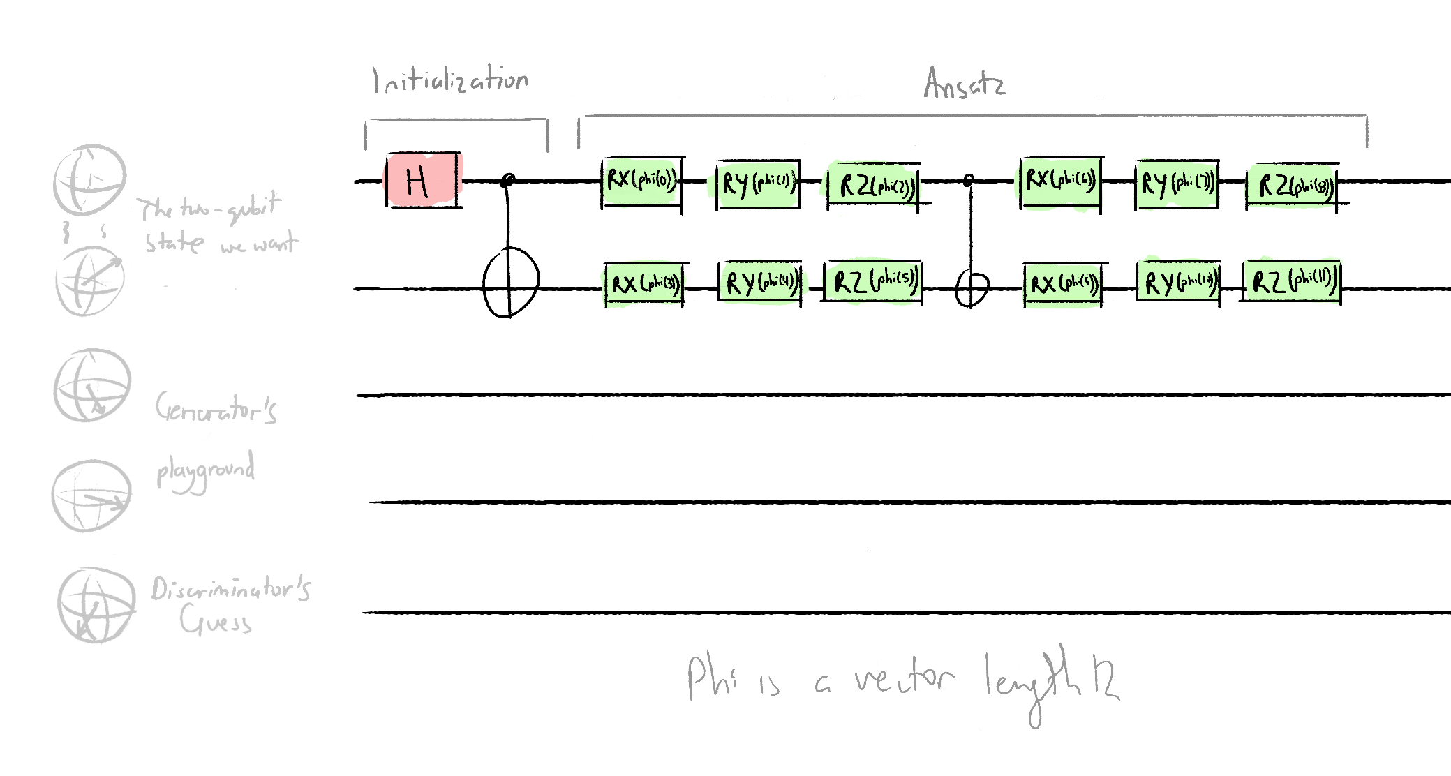
The generator QNN/parametized circuit looks like this:
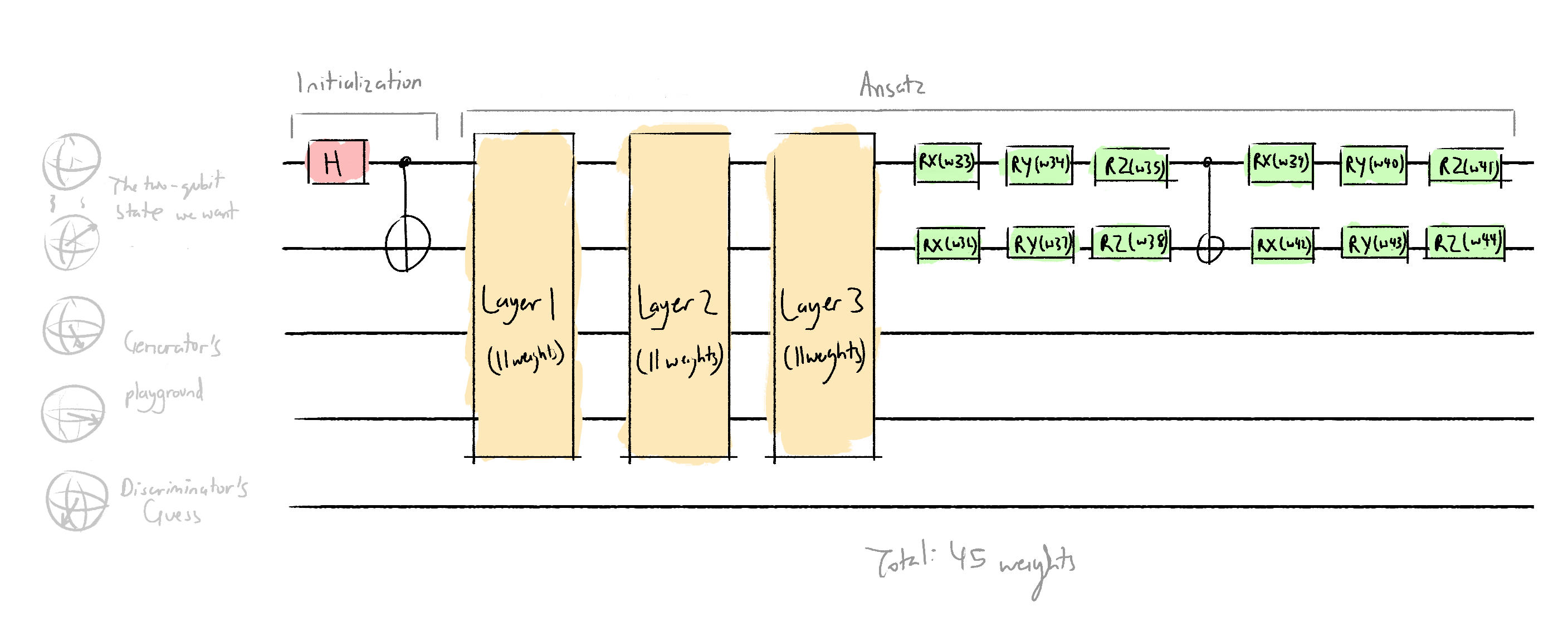
I chose to use 3 layers, quite arbitrarily, because I don't know how you're meant to choose. In the future, I can experiment with different ansatzes that have more layers. The architecture of each layer is modelled of of the proposed ansatz in Dallaire-Demers and Killoran (2018):
(Using the Pennylane printed circuit because I'm too lazy to draw my own it does the job, hence it meets speck. [^speck])
# Define the generator
# Wires 0 and 1 are the 2 qubit state.
def generator(w, **kwargs):
    qml.Hadamard(wires=0)
    qml.CNOT(wires=[0,1])
    generator_layer(w[:11])
    generator_layer(w[11:22])
    generator_layer(w[22:33]) # includes w[22], doesnt include w[33]
    qml.RX(w[33], wires=0)
    qml.RY(w[34], wires=0)
    qml.RZ(w[35], wires=0)
    qml.RX(w[36], wires=1)
    qml.RY(w[37], wires=1)
    qml.RZ(w[38], wires=1)
    qml.CNOT(wires=[0, 1])
    qml.RX(w[39], wires=0)
    qml.RY(w[40], wires=0)
    qml.RZ(w[41], wires=0)
    qml.RX(w[42], wires=1)
    qml.RY(w[43], wires=1)
    qml.RZ(w[44], wires=1)

def generator_layer(w):
    qml.RX(w[0], wires=0)
    qml.RX(w[1], wires=1)
    qml.RX(w[2], wires=2)
    qml.RX(w[3], wires=3)
    qml.RZ(w[4], wires=0)
    qml.RZ(w[5], wires=1)
    qml.RZ(w[6], wires=2)
    qml.RZ(w[7], wires=3)
    qml.MultiRZ(w[8], wires=[0, 1])
    qml.MultiRZ(w[9], wires=[2, 3])
    qml.MultiRZ(w[10], wires=[1, 2])
    # 11 weights
Here's what the discriminator architecture looks like:
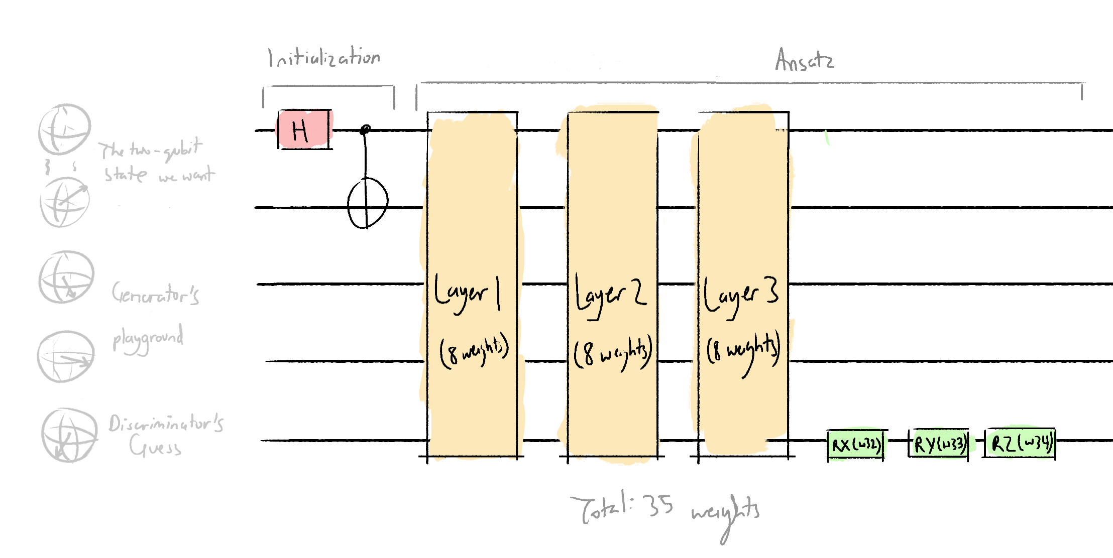
As well as each discriminator layer:
As well as the code to create that:
# The discriminator acts on wires 0, 1, and 4

def discriminator_layer(w, **kwargs):
    qml.RX(w[0], wires=0)
    qml.RX(w[1], wires=1)
    qml.RX(w[2], wires=4)
    qml.RZ(w[3], wires=0)
    qml.RZ(w[4], wires=1)
    qml.RZ(w[5], wires=4)
    qml.MultiRZ(w[6], wires=[0, 1])
    qml.MultiRZ(w[7], wires=[1, 4])

def discriminator(w, **kwargs):
    qml.Hadamard(wires=0)
    qml.CNOT(wires=[0,1])
    discriminator_layer(w[:8])
    discriminator_layer(w[8:16])
    discriminator_layer(w[16:32])
    qml.RX(w[32], wires=4)
    qml.RY(w[33], wires=4)
    qml.RZ(w[34], wires=4)
The real data circuit architecture:
# Define the real data creator
def real_data(phi, **kwargs):
    # phi is a list with length 12
    qml.Hadamard(wires=0)
    qml.CNOT(wires=[0,1])
    qml.RX(phi[0], wires=0)
    qml.RY(phi[1], wires=0)
    qml.RZ(phi[2], wires=0)
    qml.RX(phi[3], wires=0)
    qml.RY(phi[4], wires=0)
    qml.RZ(phi[5], wires=0)
    qml.CNOT(wires=[0, 1])
    qml.RX(phi[6], wires=1)
    qml.RY(phi[7], wires=1)
    qml.RZ(phi[8], wires=1)
    qml.RX(phi[9], wires=1)
    qml.RY(phi[10], wires=1)
    qml.RZ(phi[11], wires=1)
We will use two quantum nodes, just like what we did in the GAN to generate a single qubit state, and just like what we do in all GANs:
Realdata-discriminator circuit - this circuit will output an expectation value that is proportional to the probability of the discriminator classifying real data as real
Generator-discriminator circuit - this circuit will output an expectation value that is proportional to the probability of the discriminator classifying fake data as real
We return the expectation value of the wire 4 for both QNodes. In the Pennylane tutorial, the expectation value was taken in the z basis. I don't know why the z basis was chosen or why it was chosen, but to play it safe, I also used the z basis in my model.
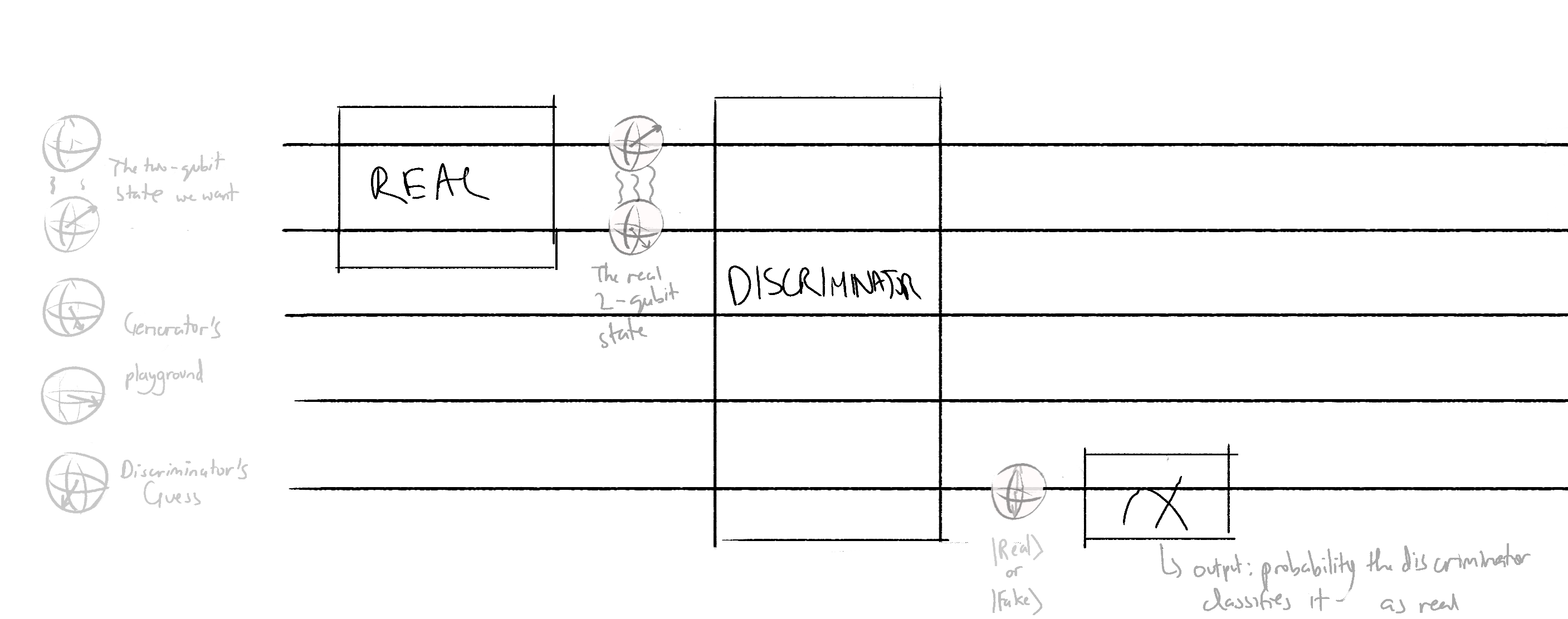
To build these QNodes:
@qml.qnode(dev, interface='tf')
def real_discriminator(phi, discriminator_weights):
    real_data(phi)
    discriminator(discriminator_weights)
    return qml.expval(qml.PauliZ(4))

@qml.qnode(dev, interface='tf')
def generator_discriminator(generator_weights, discriminator_weights):
    generator(generator_weights)
    discriminator(discriminator_weights)
    return qml.expval(qml.PauliZ(4))
The circuit architecture is done!
Cost Functions
We will need two cost functions: one for training the generator, and one for training the discriminator. These are defined in the same way as the ones used to generate a single-qubit state:
The discriminator is trying to maximize correct guesses and minimize incorrect ones. The accuracy of the discriminator is given by the probability of the discriminator classifying real data as real - the probability of the discriminator classifying fake data as real, and thus, the cost function will be QNode2 output - QNode1 ouptut.
The generator is trying to maximize how much it can fool the generator, so its accuracy is given by the probability of the discriminator classifying fake data as real, and its cost function would just be the additive inverse of that, aka the QNode2 output.
def probability_real_real(discriminator_weights):
    # probability of guessing real data as real
    discriminator_output = real_discriminator(phi, discriminator_weights)
    probability_real_real = (discriminator_output + 1) / 2
    return probability_real_real

def probability_fake_real(generator_weights, discriminator_weights):
    # probability of guessing real fake as real
    discriminator_output = generator_discriminator(generator_weights, discriminator_weights)
    probability_fake_real = (discriminator_output + 1) / 2
    return probability_fake_real

def discriminator_cost(discriminator_weights):
    accuracy = probability_real_real(discriminator_weights) - probability_fake_real(generator_weights, discriminator_weights)
    cost = -accuracy
    return cost

def generator_cost(generator_weights):
    accuracy = probability_fake_real(generator_weights, discriminator_weights)
    cost = -accuracy
    return cost
The cost functions are done!
Training, aka Optimization
We define the weights and turn them into Tensorflow-objects, because Tensorflow optimizers need their parameters to be Tensorflow-type objects.
# variables
phi = [np.pi] * 12
for i in range(len(phi)):
    phi[i] = phi[i] / np.random.randint(2, 11)
num_epochs = 30
eps = 1

initial_generator_weights = np.array([np.pi] + [0] * 44) + \
    np.random.normal(scale=eps, size=(45,))
initial_discriminator_weights = np.random.normal(scale=eps, size=(35,))

generator_weights = tf.Variable(initial_generator_weights)
discriminator_weights = tf.Variable(initial_discriminator_weights)
# Let's run some tests first to make sure the circuitry works.
print(len(initial_discriminator_weights))
print('\nCost:', discriminator_cost(discriminator_weights).numpy())
print('\nProbability classify real as real: ', probability_real_real(generator_weights).numpy())
print('\nProbability classify fake as real: ', probability_fake_real(generator_weights, discriminator_weights).numpy())
35

Cost: 0.019803181290626526

Probability classify real as real:  0.45531943440437317

Probability classify fake as real:  0.8116009086370468
Declare our Tensorflow optimizer:
opt = tf.keras.optimizers.SGD(0.4)
To make it easy to train the generator and discriminator against each other, we will define functions:
def train_discriminator():
    for epoch in range(num_epochs):
        cost = lambda: discriminator_cost(discriminator_weights) # you need "lambda" because discriminator_weights is a Tensorflow object
        opt.minimize(cost, discriminator_weights)
        if epoch % 5 == 0:
            cost_val = discriminator_cost(discriminator_weights).numpy()
            print('Epoch  {}/{}, Cost: {}, Probability class real as real: {}'.format(epoch, num_epochs, cost_val, probability_real_real(discriminator_weights).numpy()))
        if epoch == num_epochs - 1:
            print('\n')

def train_generator():
    for epoch in range(num_epochs):
        cost = lambda: generator_cost(generator_weights)
        opt.minimize(cost, generator_weights)
        if epoch % 5 == 0:
            cost_val = generator_cost(generator_weights).numpy()
            print('Epoch  {}/{}, Cost: {}, Probability class fake as real: {}'.format(epoch, num_epochs, cost_val, probability_fake_real(generator_weights, discriminator_weights).numpy()))
        if epoch == num_epochs - 1:
            print('\n')
Now it's time for the fun part, what all this work was for! Start putting the discriminator and generator to war by training them against each other:
train_discriminator()
train_generator()
Epoch  0/30, Cost: 0.016384251415729523, Probability class real as real: 0.8018914610147476
Epoch  5/30, Cost: 0.0025900080800056458, Probability class real as real: 0.8397957384586334
Epoch  10/30, Cost: -0.013791278004646301, Probability class real as real: 0.8585737869143486
Epoch  15/30, Cost: -0.05114398151636124, Probability class real as real: 0.8515666350722313
Epoch  20/30, Cost: -0.1774560660123825, Probability class real as real: 0.8271761536598206
Epoch  25/30, Cost: -0.47456610575318336, Probability class real as real: 0.9079123623669147


Epoch  0/30, Cost: -0.5134937018156052, Probability class fake as real: 0.5134937018156052
Epoch  5/30, Cost: -0.9647348411381245, Probability class fake as real: 0.9647348411381245
Epoch  10/30, Cost: -0.9905945546925068, Probability class fake as real: 0.9905945546925068
Epoch  15/30, Cost: -0.9939185006078333, Probability class fake as real: 0.9939185006078333
Epoch  20/30, Cost: -0.9952942144591361, Probability class fake as real: 0.9952942144591361
Epoch  25/30, Cost: -0.9961031721904874, Probability class fake as real: 0.9961031721904874
And again:
train_discriminator()
train_generator()
Epoch  0/30, Cost: 0.013085490791127086, Probability class real as real: 0.9817191222682595
Epoch  5/30, Cost: -0.05683990567922592, Probability class real as real: 0.9347136579453945
Epoch  10/30, Cost: -0.28723930567502975, Probability class real as real: 0.7926171645522118
Epoch  15/30, Cost: -0.7114340290427208, Probability class real as real: 0.8490715846419334
Epoch  20/30, Cost: -0.7902502901852131, Probability class real as real: 0.8959890566766262
Epoch  25/30, Cost: -0.8010090216994286, Probability class real as real: 0.9103046432137489


Epoch  0/30, Cost: -0.22221961617469788, Probability class fake as real: 0.22221961617469788
Epoch  5/30, Cost: -0.9474421814084053, Probability class fake as real: 0.9474421814084053
Epoch  10/30, Cost: -0.9798047197982669, Probability class fake as real: 0.9798047197982669
Epoch  15/30, Cost: -0.9853136069141328, Probability class fake as real: 0.9853136069141328
Epoch  20/30, Cost: -0.9882683400064707, Probability class fake as real: 0.9882683400064707
Epoch  25/30, Cost: -0.990305517334491, Probability class fake as real: 0.990305517334491
You can keep pitting these circuits against each other for as many times as you want! As for me, I'll be satisfied with a 91% discriminator accuracy and 99% generator accuracy.
Validation
obs = [qml.PauliX(0), qml.PauliY(0), qml.PauliZ(0), qml.PauliX(1), qml.PauliY(1), qml.PauliZ(1)] # the observation matrix - you measure both qubits 0 and 1 in the PauliX, PauliY, and PauliZ bases

bloch_vector_real = qml.map(real_data, obs, dev, interface="tf") # creates a QNode collection
bloch_vector_generator = qml.map(generator, obs, dev, interface="tf")

bloch_vector_realz = bloch_vector_real(phi) # here: you pass phi through the QNode collection
bloch_vector_generatorz = bloch_vector_generator(generator_weights) # calling it with a bloch_vector_generatorz at the end because adding _2 at the end is boring.

difference = np.absolute(bloch_vector_generatorz - bloch_vector_realz)
accuracy = difference / (np.pi) # It is divided by pi and not 2pi because a rotation of pi is maximum far-away-ness.

# Find the mean of the accuracy
average_accuracy = 0
for i in range(len(accuracy)):
    average_accuracy += accuracy[i]
average_accuracy = average_accuracy / len(accuracy)
average_accuracy = 1 - average_accuracy

print("Real Bloch vector: {}".format(bloch_vector_realz))
print('')
print("Generator Bloch vector: {}".format(bloch_vector_generatorz))
print('')
print("Difference: {}".format(difference))
print('')
print("Accuracy: {}".format(average_accuracy))
Real Bloch vector: [ 4.49031681e-01  8.68634649e-01  1.49011612e-07 -7.46617287e-01
  5.78252882e-01 -2.53656507e-01]

Generator Bloch vector: [ 0.32962847  0.81327445  0.24301034 -0.68318889  0.49043131 -0.35765988]

Difference: [0.11940321 0.0553602  0.24301019 0.0634284  0.08782157 0.10400337]

Accuracy: 0.9642948114019914
How that average_accuracy variable should be read is not that it is 96% accurate but that the generated two-qubit-state is within a 4% standard deviation away from the real state.
I wrote a blog post to explain why the above code is successful at retreiving the Bloch vectors.
With that, we have successfully generated the two-qubit state!
Footnote
[^speck]: Speck is an idea that Seth Godin talks about which states that the definition of whether something is high quality is if it meets speck. If your work has met speck, yes, it can be made better, but there's no point of making it any better.
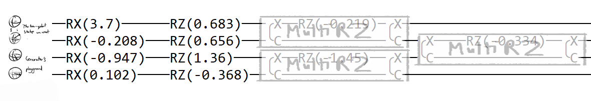
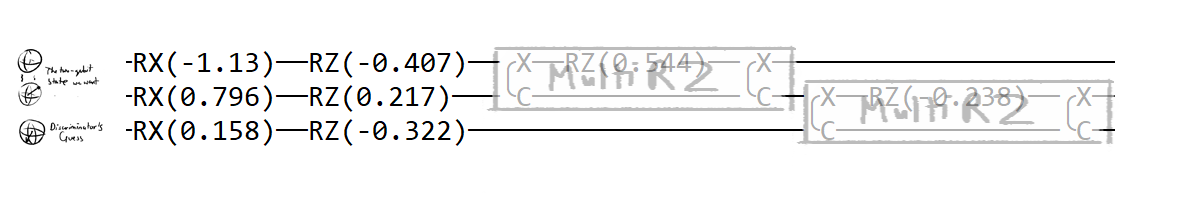
# To see the visual representation of what the discriminator and generator circuits look like

@qml.qnode(dev, interface='tf')
def generator_1(generator_weights):
    generator(generator_weights)
    return qml.expval(qml.PauliZ(1)), qml.expval(qml.PauliZ(0))


@qml.qnode(dev, interface='tf')
def discriminator_1(generator_weights):
    discriminator(generator_weights)
    return qml.expval(qml.PauliZ(1)), qml.expval(qml.PauliZ(0))

discriminator_1(discriminator_weights)
generator_1(generator_weights)
print(discriminator_1.draw())
print('\n')
print(generator_1.draw())
 0: ──H──────────╭C──────────RX(-1.66)───RZ(1.53)───╭X──RZ(-1.08)──╭X───RX(0.749)──RZ(-0.837)──────────────────────────────╭X──RZ(-1.54)──╭X───RX(0.117)──RZ(-0.677)──────────────────────────────╭X──RZ(-1.78)──╭X────────────────────────────────────────────────────┤ ⟨Z⟩
 1: ─────────────╰X──────────RX(-0.889)──RZ(-0.18)──╰C─────────────╰C──╭X──────────RZ(-1.61)───╭X──RX(-1.52)──RZ(1.76)─────╰C─────────────╰C──╭X──────────RZ(0.692)───╭X──RX(1.45)─────RZ(-2.31)──╰C─────────────╰C──╭X──RZ(-1.8)──╭X──────────────────────────────────┤ ⟨Z⟩
 4: ──RX(-1.56)───RZ(0.197)────────────────────────────────────────────╰C──────────────────────╰C──RX(0.792)──RZ(-0.0952)─────────────────────╰C──────────────────────╰C──RX(-0.0266)──RZ(2.14)──────────────────────╰C────────────╰C──RX(-1.47)──RY(1.26)──RZ(0.533)──┤


 0: ──H────────────╭C────────────RX(2.06)──RZ(-0.694)──╭X──RZ(-0.639)──╭X────────────RX(-4.13)──RZ(-0.657)───────────────────────────╭X──RZ(-0.457)──╭X───RX(-0.197)──RZ(0.521)───────────────────────────────╭X──RZ(-0.651)──╭X───RX(1.57)──RY(-0.448)───RZ(2.33)──────────────────────────────────╭C──RX(0.749)──RY(-0.542)──RZ(1.48)───┤ ⟨Z⟩
 1: ───────────────╰X────────────RX(1.02)──RZ(-0.178)──╰C──────────────╰C───────────╭X──────────RZ(-0.275)──╭X──RX(0.371)──RZ(1.2)───╰C──────────────╰C──╭X───────────RZ(-2.9)────╭X──RX(-0.176)──RZ(-0.92)───╰C──────────────╰C──╭X─────────RZ(0.179)───╭X─────────RX(1.34)──RY(0.343)──RZ(0.367)──╰X──RX(1.27)───RY(-0.546)──RZ(-1.72)──┤ ⟨Z⟩
 2: ──RX(-1.68)─────RZ(1.67)────╭X─────────RZ(1.13)────╭X───────────────────────────╰C──────────────────────╰C──RX(0.635)──RZ(0.84)──╭X──RZ(0.586)───╭X──╰C───────────────────────╰C──RX(-0.319)──RZ(-0.774)──╭X──RZ(0.144)───╭X──╰C─────────────────────╰C───────────────────────────────────────────────────────────────────────────────┤
 3: ──RX(-0.0904)───RZ(-0.625)──╰C─────────────────────╰C──RX(0.388)────RZ(-0.222)───────────────────────────────────────────────────╰C──────────────╰C───RX(1.19)────RZ(-0.114)──────────────────────────────╰C──────────────╰C──────────────────────────────────────────────────────────────────────────────────────────────────────────┤