Jupyter-first courses: Section 2 (What)
Lorena A. Barba, April 2019
Jupyter for Teaching and Learning
What is Jupyter?
Project Jupyter is a broad collaboration that develops open-source tools for interactive and exploratory computing. The tools include: IPython, the Jupyter Notebook, Jupyter Hub, and an ecosystem of extensions contributed by a large community.
The Jupyter Notebook is an application for creating interactive computational narratives. It has exploded in popularity, fueled by its adoption as the favorite environment for data science.
On May 2nd, 2018, the Association for Computing Machinery (ACM) announced that Jupyter was being awarded the prestigious ACM Software System Award. Past recipients of this award include: Unix, TeX, the World Wide Web, Java, and the GCC compiler. The ACM press release for the award says of Jupyter that it has “become a de facto standard for data analysis in research, education, journalism and industry.”
In the last three years, industry adoption of Jupyter took hold, with new products by Google (Cloud DataLab), Microsoft (AzureML, HDInsight), Intel (Trusted Analytics Platform), and IBM (IBM Watson Studio).
In April 2018, the number of publicly available Jupyter notebooks on GitHub surpassed two million, and the number crossed the three million mark in November.
Jupyter is also skyrocketing as a platform to teach computing and data science. A Gallery of Interesting Jupyter Notebooks lists entire books, lessons or courses using Jupyter for introductory programming, statistics, machine learning, mathematics, physics, signal processing, linguistics, chemistry, text mining, biomechanics, and more.
The Jupyter Notebook is a browser-based application that allows instructors to create and share documents with live equations, visualizations, and code. Jupyter Notebooks help students get started with analysis faster and provide a standardized, replicable analytic environment for shared exploration and research through interactive computing.
The Berkeley Data Science program for undergraduates, which began in Fall 2015, is entirely Jupyter-based. More than 1,000 first-year students are currently in the program, after a rapid escalation from the pilot course with 100 students. The article The Course of the Future and the Technology Behind It explains how Jupyter enabled the scaling out of the program: through “browser-based computation, avoiding the need for students to install software, transfer files, or update libraries.” This is powered by JupyterHub, a cloud-hosted version of Jupyter that universities can deploy to offer a common computational environment for all instructors and students.
The precursor of Jupyter was IPython, created by Fernando Pérez starting 2001. He says:
The role of Jupyter is to give students, researchers, journalists or industry engineers tools that give them a coherent handle on the entire process of computational exploration and discovery. We have built it so the same tools are used for individual data analysis or to create a published article, course or book.
Working in Jupyter
Several things may be counter-intuitive to you at first. For example, most people are used to launching apps in their computers by clicking some icon: this is the first thing to "unlearn." Jupyter is typically launched from the command line (like when you launched IPython). If you are using the Anaconda distribution (highly recommended), you can also open Jupyter from the Anaconda Navigator in the more familiar way of clicking an icon.
On a Jupyter notebook, you have two types of content—code and markdown—that handle a bit differently. The fact that your browser is an interface to a compute engine (called "kernel") leads to some extra housekeeping (like shutting down the kernel). But you'll get used to it pretty quick!
Start Jupyter
The standard way to start Jupyter is to type the following in the command-line interface:
jupyter notebook
Hit enter and tadah!! After a little set up time, your default browser will open with the Jupyter app. It should look like in the screenshot below, but you may see a list of files and folders, depending on the location of your computer where you launched it.
Note:
Don't close the terminal window where you launched Jupyter (while you're still working on Jupyter). If you need to do other tasks on the command line, open a new terminal window.
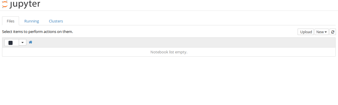 #### Screenshot of the Jupyter dashboard, open in the browser.
To start a new Jupyter notebook, click on the top-right, where it says New, and select Python 3. Check out the screenshot below.
 #### Screenshot showing how to create a new notebook.
A new tab will appear in your browser and you will see an empty notebook, with a single input line, waiting for you to enter some code. See the next screenshot.
 #### Screenshot showing an empty new notebook.
The notebook opens by default with a single empty code cell. Try to write some Python code there and execute it by hitting [shift] + [enter].
Notebook cells
The Jupyter notebook uses cells: blocks that divide chunks of text and code. Any text content is entered in a Markdown cell: it contains text that you can format using simple markers to get headings, bold, italic, bullet points, hyperlinks, and more.
Markdown is easy to learn, check out the syntax in the "Daring Fireball" webpage (by John Gruber). A few tips:
- to create a title, use a hash to start the line:
# Title - to create the next heading, use two hashes (and so on):
## Heading - to italicize a word or phrase, enclose it in asterisks (or underdashes):
*italic*or_italic_ - to make it bold, enclose it with two asterisks:
**bolded** - to make a hyperlink, use square and round brackets:
[hyperlinked text](url)
Computable content is entered in code cells. We will be using the IPython kernel ("kernel" is the name used for the computing engine), but you should know that Jupyter can be used with many different computing languages. It's amazing.
A code cell will show you an input mark, like this:
In [ ]:
Once you add some code and execute it, Jupyter will add a number ID to the input cell, and produce an output marked like this:
Out [1]:
A bit of history:
Markdown was co-created by the legendary but tragic Aaron Swartz. The biographical documentary about him is called "The Internet's Own Boy," and you can view it in YouTube or Netflix. Recommended!
Interactive computing in the notebook
Look at the icons on the menu of Jupyter (see the screenshots above). The first icon on the left (an old floppy disk) is for saving your notebook. You can add a new cell with the big + button. Then you have the cut, copy, and paste buttons. The arrows are to move your current cell up or down. Then you have a button to "run" a code cell (execute the code), the square icon means "stop" and the swirly arrow is to "restart" your notebook's kernel (if the computation is stuck, for example). Next to that, you have the cell-type selector: Code or Markdown (or others that you can ignore for now).
You can test-drive a code cell by writing some arithmetic operations. Like we saw in our first lesson, the Python operators are:
+ - * / ** % //
There's addition, subtraction, multiplication and division. The last three operators are exponent (raise to the power of), modulo (divide and return remainder) and floor division.
Typing [shift] + [enter] will execute the cell and give you the output in a new line, labeled Out[1] (the numbering increases each time you execute a cell).
Try it!
Add a cell with the plus button, enter some operations, and [shift] + [enter] to execute.
Edit mode and Command mode
Once you click on a notebook cell to select it, you may interact with it in two ways, which are called modes. Later on, when you are reviewing this material again, read more about this in Reference 1.
Edit mode:
We enter edit mode by pressing
Enteror double-clicking on the cell.We know we are in this mode when we see a green cell border and a prompt in the cell area.
When we are in edit mode, we can type into the cell, like a normal text editor.
Command mode:
We enter in command mode by pressing
Escor clicking outside the cell area.We know we are in this mode when we see a grey cell border with a left blue margin.
In this mode, certain keys are mapped to shortcuts to help with common actions.
You can find a list of the shortcuts by selecting Help->Keyboard Shortcuts
from the notebook menu bar. You may want to leave this for later, and come back to it, but it becomes more helpful the more you use Jupyter.
How to shut down the kernel and exit
Closing the browser tab where you've been working on a notebook does not immediately "shut down" the compute kernel. So you sometimes need to do a little housekeeping.
Once you close a notebook, you will see in the main Jupyter app that your notebook file has a green book symbol next to it. You should click in the box at the left of that symbol, and then click where it says Shutdown. You don't need to do this all the time, but if you have a lot of notebooks running, they will use resources in your machine.
Similarly, Jupyter is still running even after you close the tab that has the Jupyter dashboard open. To exit the Jupyter app, you should go to the terminal that you used to open Jupyter, and type [Ctrl] + [c] to exit.
Nbviewer
Nbviewer is a free web service that allows you to share static versions of hosted notebook files, as if they were a web page. If a notebook file is publicly available on the web, you can view it by entering its URL in the nbviewer web page, and hitting the Go! button. The notebook will be rendered as a static page: visitors can read everything, but they cannot interact with the code.