![]()

Exploring the New Eager Execution TensorFlow API
import tensorflow as tf
import numpy as np
import matplotlib.pyplot as plt
from mpl_toolkits.axes_grid1 import ImageGrid
from tensorflow.examples.tutorials.mnist import input_data
from keras.datasets import mnist
from sklearn.model_selection import train_test_split
from sklearn.metrics import accuracy_score
import keras
plt.rcParams["axes.grid"] = False
Using TensorFlow backend.
Deep Learning
Deep Learning is a branch of machine learning focused on building algorithms that learn data representations (instead of task-specific solutions)
Deep Learning is state-of-the-art in almost all perception problem:
- Natural Language Processing (NLP)
- Voice Recognition
- Computer Vision
![]()
Deep Learning is a family of methods:
- Feedforward Network
- Convolutional Nets
- Recurrent Nets
- Auto-Encoders
- Generative Adversarial Networks
- etc...
TensorFlow Eager Execution
Eager execution is a new high-level TF API that lets users execute tensors in real time (Imperative) fashion.
- Brings TF to the level of some other Deep Learning frameworks like PyTorch and Chainer.
- Run TF models just like any other python code (Numpy and python objects compliant)
- Don't think about Computational Graphs - Just execute code normally
- Allows for real-time python Debugging
- To enable Eager Execution - just run: tf.enable_eager_execution()
Exercise
1- Enable eager execution mode using tf.enable_eager_execution().
# Enable eager execution mode
tfe = tf.contrib.eager

## YOUR CODE GOES HERE
tf.enable_eager_execution()
if tf.executing_eagerly():
    print("Eager is Enabled!")
Eager is Enabled!
Computer Vision 101 with MNIST
Exploring the MNIST dataset
Computer Vision is a branch of AI devoted to building algorithms that enable machines to perceive the world.
MNIST is a computer vision dataset.
It contains greyscale images of handwritten digits like these.
The MNIST dataset is composed of 60000 thousand images. 50000 for training and 10000 for testing.

Numerical Stabilization
Any time we are up to doing some calculus on a computer, we need to think about representation.
- We all know, machines are memory-limited
Exercise
Accessing numerical error.
- Create two variables a and b.
- Assign 1000000000 (one billion) to a and 0.000001 to be
- In the loop add b to a 1000000 (one million) times
What happens? What should the result be?
a = 1000000000 # one billion
b = 0.000001
for i in range(1000000):
  a += b

print("a:", a)
print("a - 1000000000:", a - 1000000000)
print("Error:", 1 - (a - 1000000000))
a: 1000000000.9536743
a - 1000000000: 0.95367431640625
Error: 0.04632568359375
Try now to substitute the 1000000000 (one billion) to just one.
What do you see?
When calculating the grandients and the loss, we do NOT want their values to get too BIG or too SMALL.
- Facilitates the job of the optimizer (find the best spot in the error function)
- Makes convergence FASTER and reduces the probability of DIVERGENCE.
That is why normalization is important.
Load MNIST data
# Download the mnist data
(X_train, y_train), (X_test, y_test) = mnist.load_data()
Exercise
Like we did before, divide the training data into train and validation sets.
- You may use: train_test_split().
- Choose a reasonable value for the split fraction.
## YOUR CODE GOES HERE
X_train, X_val, y_train, y_val = train_test_split(X_train, y_train, test_size=0.1, random_state=42)
Visualize the dataset Shapes
print("Train shape:", X_train.shape)
print("Train labels:", y_train.shape)
print("Validation shape:", X_val.shape)
print("Validation labels:", y_val.shape)
print("Test shape:", X_test.shape)
print("Test labels:", y_test.shape)
Train shape: (54000, 28, 28)
Train labels: (54000,)
Validation shape: (6000, 28, 28)
Validation labels: (6000,)
Test shape: (10000, 28, 28)
Test labels: (10000,)
Exercise
Build the normalizer() function above.
Our goal is to keep the input values (pixels) in a small range.
- Option 1: Dvide the image pixels by 255. What does it mean?
- Option 2: Subtract each pixel by 128 and divide by 128.
def normalizer(image, label):
  """
  TODO: Finish the normalizer function
  """
  return 2 * tf.to_float(image) / 255. - 1.0, label
## Visualize the dataset distribution
import pylab as P
n, bins, patches = P.hist(y_train, bins=10, histtype="bar", rwidth=0.8)
print("Train:", n)
n, bins, patches = P.hist(y_test, bins=10, histtype="bar", rwidth=0.8 )
print("Test:", n)
P.xlabel('Classes')
P.ylabel('Distribution')
P.title('Train/Test distribution')
P.show()
Train: [5299. 6088. 5386. 5542. 5262. 4870. 5338. 5632. 5266. 5317.]
Test: [ 980. 1135. 1032. 1010.  982.  892.  958. 1028.  974. 1009.]

print("Max value:", np.max(X_train[0]))
print("Min value:", np.min(X_train[0]))
print("Mean:", np.mean(X_train[0]))
print("Std:", np.std(X_train[0]))
Max value: 255
Min value: 0
Mean: 11.565051020408163
Std: 45.77647391710191
Visualize some MNIST images
fig = plt.figure(1, (6., 6.))
grid = ImageGrid(fig, 111,  # similar to subplot(111)
                 nrows_ncols=(4, 4),  # creates 2x2 grid of axes
                 axes_pad=0.1,  # pad between axes in inch.
                 )

for i in range(16):
    grid[i].imshow(X_train[i], cmap="gray")  # The AxesGrid object work as a list of axes.

plt.show()

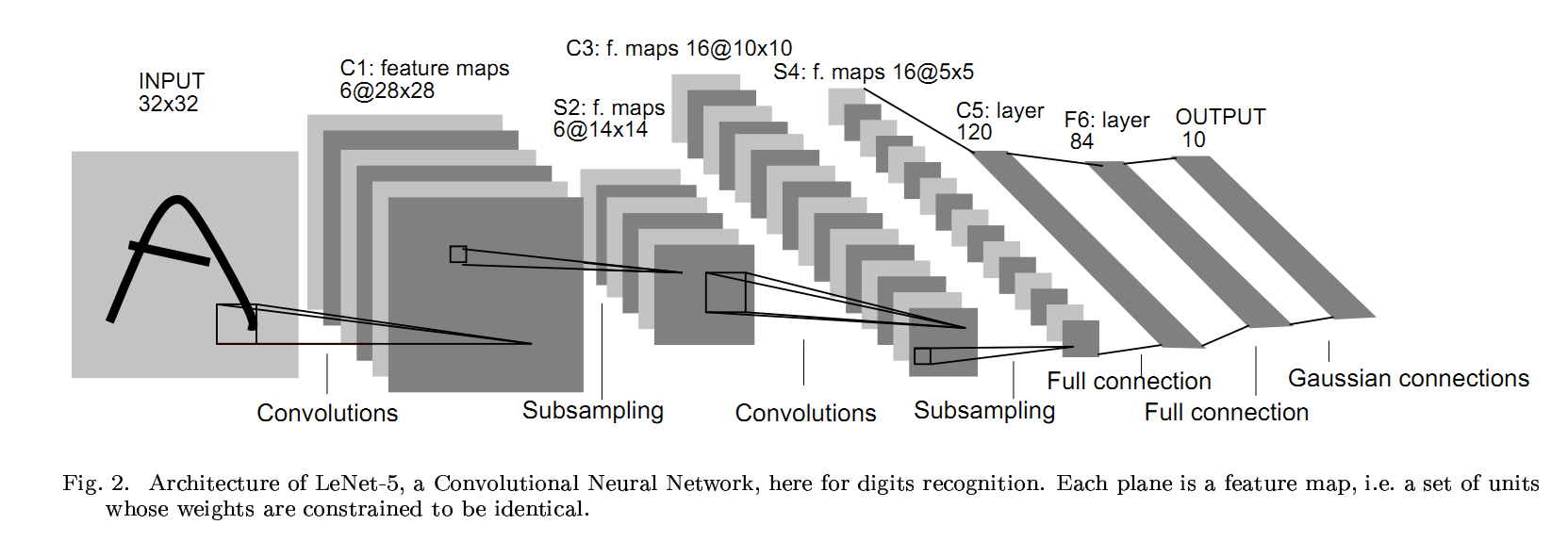
Building our Neural Net
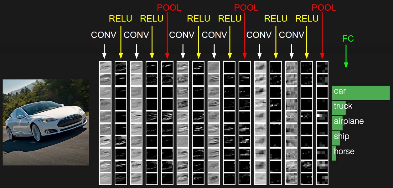
The basic architecture follows a simple sequence of operations.
- Convolution
- Activation function
- Pooling
- Fully-Connected layers
In the end, to build the classification layer, we usually use a fully-connected layer.
Refer to these links for full documentations:
Convolutions and Non-linearity
The convolution is a linear operation that uses small local receptive fields that pass over an image to create feature maps between the input and the next layer.
Its main advantage is that we do not need to engineer the features (filter).
- The network will learn them for us.
Also, Convolution are very memory efficient.
- They share parameters across space.

Non-linearity is what makes DNN cool.
ReLU (rectified linear Unit) is one of the most simple functions one can think of.
- Yet, they do just what we need. Non-linearity and Differentiability.

Exercise:
Build your own DNN using eager execution.
Hint: Use the Keras layers built into Tensorflow.
Convolutional Net template:
# def ConvNet():
#   Conv()
#   Pooling()
#   Conv()
#   Pooling()
#   ...
#   Flatten()
#   Dense()
#   Dense()
#   ...
#   Classification layer - Dense()
tf.keras.layers.Conv2D(filters, kernel_size, strides, padding, activation=tf.nn.relu, use_bias)
- filters: Number of convolutional filters. Can be 16, 32, 48 .
- kernel_size: The size of the filter. Usually 3, or 5.
- strides: Number of pixels that the filter should skip. Usually 1 or 2 (if 2, the output will have a smaller size).
- padding: One of 'same' or 'valid'. Valid padding means no padding.
tf.keras.layers.MaxPool2D(pool_size, strides=2, padding='same')
Used to reduce the features spatial dimensions.
pool_size: Size of the pooling window. Usually, 2
strides: Go with 2.
padding: Go with 'same'. We want to reduce the feature vectors dimensions!
tf.keras.layers.Dense(units=128, activation=tf.nn.relu)
- units: Number of neuron units: 96, 128, 256, 512 ...
Build a last Dense layer and set the units to have the number of classes of the dataset and no Activation Function.
class MNISTModel(tf.keras.Model):

    def __init__(self):
        super(MNISTModel, self).__init__() # Call the super class constructor

        # Now define the layers of your model
        # The convolutions, ReLUs and classifications layers goes here
        # CODE GOES HERE
        self.conv1 = tf.keras.layers.Conv2D(filters=32, kernel_size=3, strides=(1, 1),
                                            padding='same', activation=tf.nn.relu, use_bias=True)
        self.pool1 = tf.keras.layers.MaxPool2D(pool_size=2, strides=2, padding="same")
        self.flatten = tf.layers.Flatten()
        self.fc1 = tf.keras.layers.Dense(units=128, activation=tf.nn.relu)
        self.logits = tf.keras.layers.Dense(units=10)

    def call(self, inputs):
        # Use the layers defined in the constructor
        # Here, we define the model hierarchical computations
        # Start by passing the inputs to the first Conv layer and chain the results to the next layers
        # CODE GOES GERE
        conv1 = self.conv1(inputs)
        pool1 = self.pool1(conv1)
        flat = self.flatten(pool1)
        fc1 = self.fc1(flat)
        logits = self.logits(fc1)
        return logits
Loss
The loss function (or objective) is responsible for measuring how good/bad our classifier is doing.
There are many loss functions.
For multiclass problems, we usually use the cross-entropy function.
The cross-entropy loss (log-loss) is used to measure the performance of a classifier that outputs probabilities.
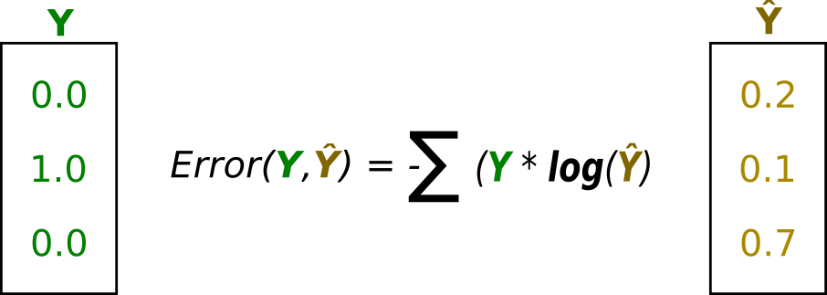
- The cross-entropy increases when the predicted value deviates from the true values and decreases otherwise.
One-hot encoding is a form of representing categorical data so that each category (class) contains the same power (magnitude) over one another.
Exercise:
Finish the loss() function bellow.
Remember, our labels are vectors. Example: [0, 3, 2, 5, 6, ..., 5].
Each number represents the image corresponding class. However, in order to make the labels equally valued, we need to convert them to binary representations (one-hot-encoding).
Use the tf.one_hot() function to convert the labels to the proper format.
For the cross-entropy loss you can choose to write it your self or use the built-in tf.nn.softmax_cross_entropy_with_logits_v2().
- If you take the challenge of writing it, tf.multiply() and tf.log() will help.
def loss(logits, labels):
  # YOUR CODE GOES HERE
  labels_one_hot = tf.one_hot(labels, 10)

  # cross_entropy = tf.nn.softmax_cross_entropy_with_logits_v2(labels=labels_one_hot, logits=logits)
  # print(cross_entropy.shape)

  cross_entropy = tf.multiply(labels_one_hot, tf.log(tf.nn.softmax(logits))) # element wise multiplication
  return - tf.reduce_mean(cross_entropy)
Exercise - Hyperparameters
Tune the hyperparameters bellow.
- Remember: The learning rate controls how fast your model learns.
- A bigger learning rate might get you to a sub-optimal objective faster, but you might overshoot the target.
## CODE GOES HERE
epochs = 1
batch_size = 32
learning_rate = 0.001
Optimizers
The Optimizer is the algorithm responsible for applying the gradients to the Model's weight variables.
Imagine a curved surface (just an example), the goal is to find the minimal value of that surface.
The Gradient points to the direction of steepest ascent. Thus, we follow the opposite direction of the gradient (steepest descent).
These are some of the Optimizers available in Tensorflow
AdadeltaOptimizer: Optimizer that implements the Adadelta algorithm.
AdagradOptimizer: Optimizer that implements the Adagrad algorithm.
AdamOptimizer: Optimizer that implements the Adam algorithm.
GradientDescentOptimizer: Optimizer that implements the gradient descent algorithm.
MomentumOptimizer: Optimizer that implements the Momentum algorithm.
Tensorflow Build-in Optimizers
Exercise:
- Pick one of these optimizers and use it to minimize the loss function for your model.
# Choose one of the optimizers and set an initial learning rate
# CODE GOES HERE
optimizer = tf.train.AdamOptimizer(learning_rate=learning_rate)
# Create the model
model = MNISTModel()
dataset = tf.data.Dataset.from_tensor_slices((X_train, y_train))
dataset = dataset.map(normalizer)
dataset = dataset.shuffle(1000) # shuffle before each epoch and bufferize some data
dataset = dataset.repeat(epochs) # number of epochs
dataset = dataset.batch(batch_size) # batch size

val_dataset = tf.data.Dataset.from_tensor_slices((X_val, y_val))
val_dataset = val_dataset.map(normalizer)
val_dataset = val_dataset.repeat(1) # number of epochs
val_dataset = val_dataset.batch(128) # batch size
Exercise
Finish the training loop. The main part is the Gradient Tape. It accumulates gradients for a batch.
Inside the GradientTape() scope:
- Compute the logits, run a forward pass through the model.
- Use the logits to compute the loss value i.e. call the loss() function.
- Outside of the GradientTape() scope compute the gradient of the loss with respect to the weights.
train_epoch_loss_avg = tfe.metrics.Mean()
train_epoch_accuracy = tfe.metrics.Accuracy()

for (step, (images, labels)) in enumerate(tfe.Iterator(dataset)):
  with tfe.GradientTape() as tape:
    # Call the model() here and pass it the input batches
    logits = model(tf.expand_dims(images, axis=3))

    # Call the loss() function - That will give you the loss signal for the given batch
    loss_value = loss(logits, labels)

  # Compute the gradient of the loss with respect to the models' weights
  grads = tape.gradient(loss_value, model.variables)

  optimizer.apply_gradients(zip(grads, model.variables),
                            global_step=tf.train.get_or_create_global_step())

  train_epoch_loss_avg(loss_value)
  train_epoch_accuracy(tf.cast(tf.argmax(logits, axis=1), tf.uint8), labels)

  if step % 100 == 0:
    val_predictions = []
    for (val_step, (val_images, val_labels)) in enumerate(tfe.Iterator(val_dataset)):
      val_logits = model(tf.expand_dims(val_images, axis=3))
      val_pred = tf.argmax(val_logits, axis=1)
      val_predictions.extend(val_pred)

    print("Training loss: {: .3}\tTrain Accuracy: {: .3}\tValidation Accuracy: {: .3}".format(train_epoch_loss_avg.result(), train_epoch_accuracy.result(), accuracy_score(val_predictions, y_val)))
Training loss:  0.178	Train Accuracy:  0.5	Validation Accuracy:  0.525
Training loss:  0.066	Train Accuracy:  0.807	Validation Accuracy:  0.888
Training loss:  0.0513	Train Accuracy:  0.848	Validation Accuracy:  0.908
Training loss:  0.0443	Train Accuracy:  0.869	Validation Accuracy:  0.915
Training loss:  0.0388	Train Accuracy:  0.887	Validation Accuracy:  0.938
Training loss:  0.0354	Train Accuracy:  0.896	Validation Accuracy:  0.947
Training loss:  0.0325	Train Accuracy:  0.904	Validation Accuracy:  0.954
Training loss:  0.0302	Train Accuracy:  0.911	Validation Accuracy:  0.96
Training loss:  0.0283	Train Accuracy:  0.917	Validation Accuracy:  0.961
Training loss:  0.0266	Train Accuracy:  0.921	Validation Accuracy:  0.963
Training loss:  0.025	Train Accuracy:  0.926	Validation Accuracy:  0.969
Training loss:  0.0237	Train Accuracy:  0.93	Validation Accuracy:  0.969
Training loss:  0.0228	Train Accuracy:  0.932	Validation Accuracy:  0.972
Training loss:  0.0221	Train Accuracy:  0.935	Validation Accuracy:  0.962
Training loss:  0.0213	Train Accuracy:  0.937	Validation Accuracy:  0.975
Training loss:  0.0207	Train Accuracy:  0.939	Validation Accuracy:  0.973
Training loss:  0.0199	Train Accuracy:  0.941	Validation Accuracy:  0.975
Training loss:  0.0193	Train Accuracy:  0.943	Validation Accuracy:  0.971
Training loss:  0.0188	Train Accuracy:  0.945	Validation Accuracy:  0.969
Training loss:  0.0182	Train Accuracy:  0.946	Validation Accuracy:  0.974
Training loss:  0.0178	Train Accuracy:  0.947	Validation Accuracy:  0.974
Training loss:  0.0174	Train Accuracy:  0.948	Validation Accuracy:  0.976
Training loss:  0.0171	Train Accuracy:  0.949	Validation Accuracy:  0.98
Training loss:  0.0168	Train Accuracy:  0.95	Validation Accuracy:  0.979
Training loss:  0.0165	Train Accuracy:  0.951	Validation Accuracy:  0.975
Training loss:  0.0161	Train Accuracy:  0.952	Validation Accuracy:  0.976
Training loss:  0.0158	Train Accuracy:  0.953	Validation Accuracy:  0.979
Training loss:  0.0154	Train Accuracy:  0.954	Validation Accuracy:  0.982
Training loss:  0.0152	Train Accuracy:  0.955	Validation Accuracy:  0.982
Training loss:  0.015	Train Accuracy:  0.955	Validation Accuracy:  0.98
Training loss:  0.0147	Train Accuracy:  0.956	Validation Accuracy:  0.979
Training loss:  0.0144	Train Accuracy:  0.957	Validation Accuracy:  0.982
Training loss:  0.0142	Train Accuracy:  0.958	Validation Accuracy:  0.98
Training loss:  0.0139	Train Accuracy:  0.958	Validation Accuracy:  0.982
from sklearn.metrics import confusion_matrix
import itertools

def plot_confusion_matrix(cm, classes,
                          normalize=False,
                          title='Confusion matrix',
                          cmap=plt.cm.Blues):
    """
    This function prints and plots the confusion matrix.
    Normalization can be applied by setting `normalize=True`.
    """
    if normalize:
        cm = cm.astype('float') / cm.sum(axis=1)[:, np.newaxis]
        print("Normalized confusion matrix")
    else:
        print('Confusion matrix, without normalization')

    # print(cm)

    plt.imshow(cm, interpolation='nearest', cmap=cmap)
    plt.title(title)
    plt.colorbar()
    tick_marks = np.arange(len(classes))
    plt.xticks(tick_marks, classes, rotation=45)
    plt.yticks(tick_marks, classes)

    fmt = '.2f' if normalize else 'd'
    thresh = cm.max() / 2.
    for i, j in itertools.product(range(cm.shape[0]), range(cm.shape[1])):
        plt.text(j, i, format(cm[i, j], fmt),
                 horizontalalignment="center",
                 color="white" if cm[i, j] > thresh else "black")

    plt.tight_layout()
    plt.ylabel('True label')
    plt.xlabel('Predicted label')
    plt.show()

def normalized_acc(conf_matrix):
    for i in range(conf_matrix.shape[0]):
        print("Acc class {0} --> {1: .3}".format(i, conf_matrix[i,i]/sum(conf_matrix[i])))
Evaluation
Run the trained model using the testing dataset.
test_dataset = tf.data.Dataset.from_tensor_slices((X_test, y_test))
test_dataset = test_dataset.map(normalizer)
test_dataset = test_dataset.repeat(1) # number of epochs
test_dataset = test_dataset.batch(128) # batch size

test_predictions = []
for (_, (test_images, test_labels)) in enumerate(tfe.Iterator(test_dataset)):
  test_logits = model(tf.expand_dims(test_images, axis=3))
  test_pred = tf.argmax(test_logits, axis=1)
  test_predictions.extend(test_pred)

print("Test Overall Accuracy: {: .3}".format(accuracy_score(test_predictions, y_test)))
Test Overall Accuracy: 0.981
conf_matrix = confusion_matrix(test_predictions, y_test)
_ = plot_confusion_matrix(conf_matrix, classes=[str(i) for i in range(10)])
Confusion matrix, without normalization

normalized_acc(conf_matrix)
Acc class 0 -->  0.959
Acc class 1 -->  0.991
Acc class 2 -->  0.981
Acc class 3 -->  0.977
Acc class 4 -->  0.99
Acc class 5 -->  0.981
Acc class 6 -->  0.995
Acc class 7 -->  0.98
Acc class 8 -->  0.97
Acc class 9 -->  0.985