ML for Gas Adsorption
-1. Only if you run this notebook on Colab
If you use this notebook on Colab, please uncomment the lines below (remove the #) and execute the cell.
#import sys
#!{sys.executable} -m pip install -U pandas-profiling[notebook]
#!jupyter nbextension enable --py widgetsnbextension
#!pip install --upgrade pandas sklearn holoviews bokeh plotly matplotlib
#!wget https://raw.githubusercontent.com/kjappelbaum/ml_molsim/2022/descriptornames.py
#!mkdir data
#!cd data && wget https://github.com/kjappelbaum/ml_molsim/raw/2022/data/data.csv
#!cd data && wget https://github.com/kjappelbaum/ml_molsim/raw/2022/data/features.csv
# import os, holoviews as hv
# os.environ['HV_DOC_HTML'] = 'true'
Import packages we will need
# basics
import os
import numpy as np
import pprint as pp

# pandas is used to read/process data
import pandas as pd

# machine learning dependencies
# scaling of data
from sklearn.preprocessing import StandardScaler, MinMaxScaler, RobustScaler
# train/test split
from sklearn.model_selection import train_test_split
# model selection
from sklearn.model_selection import GridSearchCV, RandomizedSearchCV
# the KRR model
from sklearn.kernel_ridge import KernelRidge
# linear model
from sklearn.linear_model import LinearRegression
# pipeline to streamline modeling pipelines
from sklearn.pipeline import Pipeline
# principal component analysis
from sklearn.decomposition import PCA
# polynomial kernel
from sklearn.metrics.pairwise import polynomial_kernel
# Dummy model as baseline
from sklearn.dummy import DummyClassifier, DummyRegressor
# Variance Threshold for feature selection
from sklearn.feature_selection import VarianceThreshold, SelectFromModel
# metrics to measure model performance
from sklearn.metrics import (accuracy_score, precision_score, recall_score, f1_score,
                             mean_absolute_error, mean_squared_error, max_error)

# save/load models
import joblib

# For the permutation importance implementation
from joblib import Parallel
from joblib import delayed
from sklearn.metrics import check_scoring
from sklearn.utils import Bunch
from sklearn.utils import check_random_state
from sklearn.utils import check_array

# plotting
import matplotlib.pyplot as plt
%matplotlib inline
from pymatviz.parity import hist_density

RANDOM_SEED = 4242424242
DATA_DIR = 'data'
DATA_FILE = os.path.join(DATA_DIR, 'data.csv')

np.random.seed(RANDOM_SEED)
other_descriptors = ["CellV [A^3]"]

geometric_descriptors = [
    "Di",
    "Df",
    "Dif",
    "density [g/cm^3]",
    "total_SA_volumetric",
    "total_SA_gravimetric",
    "total_POV_volumetric",
    "total_POV_gravimetric",
]

linker_descriptors = [
    "f-lig-chi-0",
    "f-lig-chi-1",
    "f-lig-chi-2",
    "f-lig-chi-3",
    "f-lig-Z-0",
    "f-lig-Z-1",
    "f-lig-Z-2",
    "f-lig-Z-3",
    "f-lig-I-0",
    "f-lig-I-1",
    "f-lig-I-2",
    "f-lig-I-3",
    "f-lig-T-0",
    "f-lig-T-1",
    "f-lig-T-2",
    "f-lig-T-3",
    "f-lig-S-0",
    "f-lig-S-1",
    "f-lig-S-2",
    "f-lig-S-3",
    "lc-chi-0-all",
    "lc-chi-1-all",
    "lc-chi-2-all",
    "lc-chi-3-all",
    "lc-Z-0-all",
    "lc-Z-1-all",
    "lc-Z-2-all",
    "lc-Z-3-all",
    "lc-I-0-all",
    "lc-I-1-all",
    "lc-I-2-all",
    "lc-I-3-all",
    "lc-T-0-all",
    "lc-T-1-all",
    "lc-T-2-all",
    "lc-T-3-all",
    "lc-S-0-all",
    "lc-S-1-all",
    "lc-S-2-all",
    "lc-S-3-all",
    "lc-alpha-0-all",
    "lc-alpha-1-all",
    "lc-alpha-2-all",
    "lc-alpha-3-all",
    "D_lc-chi-0-all",
    "D_lc-chi-1-all",
    "D_lc-chi-2-all",
    "D_lc-chi-3-all",
    "D_lc-Z-0-all",
    "D_lc-Z-1-all",
    "D_lc-Z-2-all",
    "D_lc-Z-3-all",
    "D_lc-I-0-all",
    "D_lc-I-1-all",
    "D_lc-I-2-all",
    "D_lc-I-3-all",
    "D_lc-T-0-all",
    "D_lc-T-1-all",
    "D_lc-T-2-all",
    "D_lc-T-3-all",
    "D_lc-S-0-all",
    "D_lc-S-1-all",
    "D_lc-S-2-all",
    "D_lc-S-3-all",
    "D_lc-alpha-0-all",
    "D_lc-alpha-1-all",
    "D_lc-alpha-2-all",
    "D_lc-alpha-3-all",
]

metalcenter_descriptors = [
    "mc_CRY-chi-0-all",
    "mc_CRY-chi-1-all",
    "mc_CRY-chi-2-all",
    "mc_CRY-chi-3-all",
    "mc_CRY-Z-0-all",
    "mc_CRY-Z-1-all",
    "mc_CRY-Z-2-all",
    "mc_CRY-Z-3-all",
    "mc_CRY-I-0-all",
    "mc_CRY-I-1-all",
    "mc_CRY-I-2-all",
    "mc_CRY-I-3-all",
    "mc_CRY-T-0-all",
    "mc_CRY-T-1-all",
    "mc_CRY-T-2-all",
    "mc_CRY-T-3-all",
    "mc_CRY-S-0-all",
    "mc_CRY-S-1-all",
    "mc_CRY-S-2-all",
    "mc_CRY-S-3-all",
    "D_mc_CRY-chi-0-all",
    "D_mc_CRY-chi-1-all",
    "D_mc_CRY-chi-2-all",
    "D_mc_CRY-chi-3-all",
    "D_mc_CRY-Z-0-all",
    "D_mc_CRY-Z-1-all",
    "D_mc_CRY-Z-2-all",
    "D_mc_CRY-Z-3-all",
    "D_mc_CRY-I-0-all",
    "D_mc_CRY-I-1-all",
    "D_mc_CRY-I-2-all",
    "D_mc_CRY-I-3-all",
    "D_mc_CRY-T-0-all",
    "D_mc_CRY-T-1-all",
    "D_mc_CRY-T-2-all",
    "D_mc_CRY-T-3-all",
    "D_mc_CRY-S-0-all",
    "D_mc_CRY-S-1-all",
    "D_mc_CRY-S-2-all",
    "D_mc_CRY-S-3-all",
]

functionalgroup_descriptors = [
    "func-chi-0-all",
    "func-chi-1-all",
    "func-chi-2-all",
    "func-chi-3-all",
    "func-Z-0-all",
    "func-Z-1-all",
    "func-Z-2-all",
    "func-Z-3-all",
    "func-I-0-all",
    "func-I-1-all",
    "func-I-2-all",
    "func-I-3-all",
    "func-T-0-all",
    "func-T-1-all",
    "func-T-2-all",
    "func-T-3-all",
    "func-S-0-all",
    "func-S-1-all",
    "func-S-2-all",
    "func-S-3-all",
    "func-alpha-0-all",
    "func-alpha-1-all",
    "func-alpha-2-all",
    "func-alpha-3-all",
    "D_func-chi-0-all",
    "D_func-chi-1-all",
    "D_func-chi-2-all",
    "D_func-chi-3-all",
    "D_func-Z-0-all",
    "D_func-Z-1-all",
    "D_func-Z-2-all",
    "D_func-Z-3-all",
    "D_func-I-0-all",
    "D_func-I-1-all",
    "D_func-I-2-all",
    "D_func-I-3-all",
    "D_func-T-0-all",
    "D_func-T-1-all",
    "D_func-T-2-all",
    "D_func-T-3-all",
    "D_func-S-0-all",
    "D_func-S-1-all",
    "D_func-S-2-all",
    "D_func-S-3-all",
    "D_func-alpha-0-all",
    "D_func-alpha-1-all",
    "D_func-alpha-2-all",
    "D_func-alpha-3-all",
]


summed_linker_descriptors = [
    "sum-f-lig-chi-0",
    "sum-f-lig-chi-1",
    "sum-f-lig-chi-2",
    "sum-f-lig-chi-3",
    "sum-f-lig-Z-0",
    "sum-f-lig-Z-1",
    "sum-f-lig-Z-2",
    "sum-f-lig-Z-3",
    "sum-f-lig-I-0",
    "sum-f-lig-I-1",
    "sum-f-lig-I-2",
    "sum-f-lig-I-3",
    "sum-f-lig-T-0",
    "sum-f-lig-T-1",
    "sum-f-lig-T-2",
    "sum-f-lig-T-3",
    "sum-f-lig-S-0",
    "sum-f-lig-S-1",
    "sum-f-lig-S-2",
    "sum-f-lig-S-3",
    "sum-lc-chi-0-all",
    "sum-lc-chi-1-all",
    "sum-lc-chi-2-all",
    "sum-lc-chi-3-all",
    "sum-lc-Z-0-all",
    "sum-lc-Z-1-all",
    "sum-lc-Z-2-all",
    "sum-lc-Z-3-all",
    "sum-lc-I-0-all",
    "sum-lc-I-1-all",
    "sum-lc-I-2-all",
    "sum-lc-I-3-all",
    "sum-lc-T-0-all",
    "sum-lc-T-1-all",
    "sum-lc-T-2-all",
    "sum-lc-T-3-all",
    "sum-lc-S-0-all",
    "sum-lc-S-1-all",
    "sum-lc-S-2-all",
    "sum-lc-S-3-all",
    "sum-lc-alpha-0-all",
    "sum-lc-alpha-1-all",
    "sum-lc-alpha-2-all",
    "sum-lc-alpha-3-all",
    "sum-D_lc-chi-0-all",
    "sum-D_lc-chi-1-all",
    "sum-D_lc-chi-2-all",
    "sum-D_lc-chi-3-all",
    "sum-D_lc-Z-0-all",
    "sum-D_lc-Z-1-all",
    "sum-D_lc-Z-2-all",
    "sum-D_lc-Z-3-all",
    "sum-D_lc-I-0-all",
    "sum-D_lc-I-1-all",
    "sum-D_lc-I-2-all",
    "sum-D_lc-I-3-all",
    "sum-D_lc-T-0-all",
    "sum-D_lc-T-1-all",
    "sum-D_lc-T-2-all",
    "sum-D_lc-T-3-all",
    "sum-D_lc-S-0-all",
    "sum-D_lc-S-1-all",
    "sum-D_lc-S-2-all",
    "sum-D_lc-S-3-all",
    "sum-D_lc-alpha-0-all",
    "sum-D_lc-alpha-1-all",
    "sum-D_lc-alpha-2-all",
    "sum-D_lc-alpha-3-all",
]

summed_metalcenter_descriptors = [
    "sum-mc_CRY-chi-0-all",
    "sum-mc_CRY-chi-1-all",
    "sum-mc_CRY-chi-2-all",
    "sum-mc_CRY-chi-3-all",
    "sum-mc_CRY-Z-0-all",
    "sum-mc_CRY-Z-1-all",
    "sum-mc_CRY-Z-2-all",
    "sum-mc_CRY-Z-3-all",
    "sum-mc_CRY-I-0-all",
    "sum-mc_CRY-I-1-all",
    "sum-mc_CRY-I-2-all",
    "sum-mc_CRY-I-3-all",
    "sum-mc_CRY-T-0-all",
    "sum-mc_CRY-T-1-all",
    "sum-mc_CRY-T-2-all",
    "sum-mc_CRY-T-3-all",
    "sum-mc_CRY-S-0-all",
    "sum-mc_CRY-S-1-all",
    "sum-mc_CRY-S-2-all",
    "sum-mc_CRY-S-3-all",
    "sum-D_mc_CRY-chi-0-all",
    "sum-D_mc_CRY-chi-1-all",
    "sum-D_mc_CRY-chi-2-all",
    "sum-D_mc_CRY-chi-3-all",
    "sum-D_mc_CRY-Z-0-all",
    "sum-D_mc_CRY-Z-1-all",
    "sum-D_mc_CRY-Z-2-all",
    "sum-D_mc_CRY-Z-3-all",
    "sum-D_mc_CRY-I-0-all",
    "sum-D_mc_CRY-I-1-all",
    "sum-D_mc_CRY-I-2-all",
    "sum-D_mc_CRY-I-3-all",
    "sum-D_mc_CRY-T-0-all",
    "sum-D_mc_CRY-T-1-all",
    "sum-D_mc_CRY-T-2-all",
    "sum-D_mc_CRY-T-3-all",
    "sum-D_mc_CRY-S-0-all",
    "sum-D_mc_CRY-S-1-all",
    "sum-D_mc_CRY-S-2-all",
    "sum-D_mc_CRY-S-3-all",
]

summed_functionalgroup_descriptors = [
    "sum-func-chi-0-all",
    "sum-func-chi-1-all",
    "sum-func-chi-2-all",
    "sum-func-chi-3-all",
    "sum-func-Z-0-all",
    "sum-func-Z-1-all",
    "sum-func-Z-2-all",
    "sum-func-Z-3-all",
    "sum-func-I-0-all",
    "sum-func-I-1-all",
    "sum-func-I-2-all",
    "sum-func-I-3-all",
    "sum-func-T-0-all",
    "sum-func-T-1-all",
    "sum-func-T-2-all",
    "sum-func-T-3-all",
    "sum-func-S-0-all",
    "sum-func-S-1-all",
    "sum-func-S-2-all",
    "sum-func-S-3-all",
    "sum-func-alpha-0-all",
    "sum-func-alpha-1-all",
    "sum-func-alpha-2-all",
    "sum-func-alpha-3-all",
    "sum-D_func-chi-0-all",
    "sum-D_func-chi-1-all",
    "sum-D_func-chi-2-all",
    "sum-D_func-chi-3-all",
    "sum-D_func-Z-0-all",
    "sum-D_func-Z-1-all",
    "sum-D_func-Z-2-all",
    "sum-D_func-Z-3-all",
    "sum-D_func-I-0-all",
    "sum-D_func-I-1-all",
    "sum-D_func-I-2-all",
    "sum-D_func-I-3-all",
    "sum-D_func-T-0-all",
    "sum-D_func-T-1-all",
    "sum-D_func-T-2-all",
    "sum-D_func-T-3-all",
    "sum-D_func-S-0-all",
    "sum-D_func-S-1-all",
    "sum-D_func-S-2-all",
    "sum-D_func-S-3-all",
    "sum-D_func-alpha-0-all",
    "sum-D_func-alpha-1-all",
    "sum-D_func-alpha-2-all",
    "sum-D_func-alpha-3-all",
]
$\color{DarkBlue}{\textsf{Short question}}$
- We declared a global variable to fix the random seed (
RANDOM_SEED). Why did we do this?
Hands-on Project: Carbon-dioxide uptake in MOFs
In this exercise we will build a model that can predict the CO$_2$ uptake of metal-organic frameworks (MOFs), which are crystalline materials consisting of inorganic metal nodes linked by organic linkers.

There are two main learning goals for this exercise:
Understand the typical workflow for machine learning in materials science. We will cover exploratory data analysis (EDA) and supervised learning (KRR).
Get familiar with some Python packages that are useful for data analysis and visualization.
At the end of the exercise, you will produce an interactive plot like the one below, comparing the predictions of your model against CO$_2$ computed with GCMC simulations. The histograms show the distributions of the errors on the training set (left) and on the test set (right).
This exercise requires a basic knowledge of Python, e.g. that you can write list comprehensions, and are able to read documentation of functions provided by Python packages.
You will be asked to provide some function arguments (indicated by #fillme comments).
You can execute all the following code cells by pressing SHIFT and ENTER and get informations about the functions by pressing TAB when you are between the parentheses (see the notes for more tips).
Also the sklearn documentation is a great source of reference with many explanations and examples.
In pandas dataframe (df) you can select columns using their name by running df[columnname]. If at any point you think that the dataset is too large for your computer, you can select a subset using df.sample() or by making the test set larger in the train/test split (section 2).
1. Import the data
df = pd.read_csv(DATA_FILE)
Let's take a look at the first few rows to see if everythings seems reasonable ...
df.head()
| ASA [m^2/cm^3] | CellV [A^3] | Df | Di | Dif | NASA [m^2/cm^3] | POAV [cm^3/g] | POAVF | PONAV [cm^3/g] | PONAVF | ... | pure_methane_widomHOA | pure_uptake_CO2_298.00_15000 | pure_uptake_CO2_298.00_1600000 | pure_uptake_methane_298.00_580000 | pure_uptake_methane_298.00_6500000 | logKH_CO2 | logKH_CH4 | CH4DC | CH4HPSTP | CH4LPSTP | |
|---|---|---|---|---|---|---|---|---|---|---|---|---|---|---|---|---|---|---|---|---|---|
| 0 | 2329.01 | 1251.28 | 6.61256 | 8.87694 | 8.48668 | 0.0 | 0.818919 | 0.68874 | 0.0 | 0.0 | ... | -8.144317 | 0.111981 | 14.218595 | 1.680640 | 9.163066 | -5.125451 | -5.511444 | 175.569974 | 215.005044 | 39.435070 |
| 1 | 1983.81 | 1254.01 | 5.80566 | 7.13426 | 7.13154 | 0.0 | 0.495493 | 0.58032 | 0.0 | 0.0 | ... | -10.208005 | 0.481625 | 9.312424 | 1.513152 | 5.908356 | -4.502967 | -5.505947 | 143.616349 | 193.059644 | 49.443295 |
| 2 | 2259.13 | 1250.58 | 5.99131 | 8.01682 | 7.98933 | 0.0 | 0.728036 | 0.65710 | 0.0 | 0.0 | ... | -8.479801 | 0.401683 | 14.796071 | 1.569714 | 7.933198 | -4.433968 | -5.525707 | 160.238808 | 199.765744 | 39.526937 |
| 3 | 1424.54 | 1249.27 | 4.73477 | 7.05822 | 7.05822 | 0.0 | 0.453157 | 0.47338 | 0.0 | 0.0 | ... | -12.615382 | 0.821747 | 10.816880 | 2.161833 | 6.710778 | -4.135434 | -5.297082 | 132.576623 | 195.582107 | 63.005483 |
| 4 | 2228.31 | 1250.61 | 6.40783 | 8.35944 | 8.26946 | 0.0 | 0.700539 | 0.65092 | 0.0 | 0.0 | ... | -8.743404 | 0.258905 | 14.153999 | 1.653013 | 8.272621 | -4.774301 | -5.515219 | 171.601539 | 214.452966 | 42.851427 |
5 rows × 343 columns
Click here for a hint
- Use something like
pd.options.display.max_columns=100to adjust how many columns are shown.pd.options.display.max_columns=100would show at maximum 100 columns.
Let's also get some basic information ...
df.info()
<class 'pandas.core.frame.DataFrame'>
RangeIndex: 17379 entries, 0 to 17378
Columns: 343 entries, ASA [m^2/cm^3] to CH4LPSTP
dtypes: float64(342), object(1)
memory usage: 45.5+ MB
$\color{DarkBlue}{\textsf{Short question}}$
- How many materials are in the dataset?
- Which datatypes do we deal with?
Below, we define three global variables (hence upper case), which are the names of our feature and target columns. We will use the TARGET for the actual regression and the TARGET_BINARY only for the stratified train/test split. The FEATURES variable is a list of column names of our dataframe.
TARGET = "pure_uptake_CO2_298.00_1600000"
TARGET_BINARY = "target_binned"  # will be created later
FEATURES = (
    geometric_descriptors
    + summed_functionalgroup_descriptors
    + summed_linker_descriptors
    + summed_metalcenter_descriptors
)
As descriptors we will use geometric properties such as density, pore volume, etc. and revised autocorrelation functions (RACs) that have been optimized for describing inorganic compounds (and recently adapated for MOFs)
Examples for pore geometry descriptors (in geometric_descriptors) include: $D_i$ (the size of the largest included sphere), $D_f$ (the largest free sphere), and $D_{if}$ (the largest included free sphere) along the pore $-$ three ways of characterizing pore size.

Also included are the surface area (SA) of the pore, and the probe-occupiable pore volume (POV). More details on the description of pore geometries can be found in Ongari et al.
RACs (in the lists starting with summed_...) operate on the structure graph and encode information about the metal center, linkers and the functional groups as differences or products of heuristics that are relevant for inorganic chemistry, such as electronegativity ($\chi$), connectivity ($T$), identity ($I$), covalent radii ($S$), and nuclear charge ($Z$).

The number in the descriptornames shows the coordination shell that was considered in the calculation of the RACs.
The target we use for this application is the high-pressure CO$_2$ uptake. This is the amount of CO$_2$ (mmol) the MOF can load per gram.
2. Split the data
Next, we split our data into a training set and a test set.
In order to prevent any information of the test set from leaking into our model, we split before starting to analyze or transform our data. For more details on why this matters, see chapter 7.10.2 of Elements of Statistical Learning.
2.1. Split with stratification
Stratification ensures that the class distributions (ratio of "good" to "bad" materials) are the same in the training and test set.
$\color{DarkBlue}{\textsf{Short question}}$
- Why is this important? What could happen if we would not do this?
For stratification to work, we to define what makes a "good" or a "bad" material. We will use 15 mmol CO$_2$ / g as the threshold for the uptake, thus binarizing our continuous target variable. (You can choose it based on the histogram of the variables).
$\color{DarkBlue}{\textsf{Short Exercise}}$
- add a column 'target_binary' that encodes whether a material is low performing (
0) or high perfoming (1) by comparing the uptake with theTHRESHOLD
Click here for a hint
- you can use pd.cut, list comprehension, the binarizer in sklearn ...)
- a list comprehension example:
[1 if value > THRESHOLD else 0 for value in df[TARGET]]
THRESHOLD = 15 # in units of mmol CO2/g
df[TARGET_BINARY] = # add your code
Now, we can perform the actual split into training and test set.
$\color{DarkBlue}{\textsf{Short Exercise}}$
- select reasonable values for
XXandXYand then perform the test/train splits. What do you consider when making this decision (think about what you would do with really small and really big datasets, what happens if you have only one test point, what happens to the model performance if you have more test points than training points)? - why do we need to perform the split into a training and test set?
- would we use the test set to tune the hyperparameters of our model?
Click here for a hint
- The `size` arguments can either be integers or, often more convenient, decimals like 0.1
- When you perform the split into training and test set you need to trade-off bias (pessimistic bias due to little training data) and variance (due to little test data)
- A typical split cloud be 70/30, but for huge dataset the test set might be too big and for small datasets the training set might be too small in this way
df_train_stratified, df_test_stratified = train_test_split(
    df,
    train_size=XX,
    test_size=XY,
    random_state=RANDOM_SEED,
    stratify=df[TARGET_BINARY],
)
3. Exploratory data analysis (EDA)
After we have put the test set aside, we can give the training set a closer look.
3.1. Correlations
$\color{DarkBlue}{\textsf{Short Exercise}}$
- Plot some features against the target property and calculate the Pearson and Spearman correlation coefficient (what is the different between those correlation coefficients?)
- What are the strongest correlations? Did you expect them?
- What can be a problem when features are correlated?
- Optional: Do they change if you switch from CO$_2$ to CH$_4$ uptake as the target instead? Explain your observation.
To get the correlation matrices, you can use the df.corr(method=)method on your dataframe (df). You might want to calculate not the full correlation matrix but just the correlation of the features with the targets
Click here for a hint
- To get the correlation with a target, you can use indexing. E.g.
df.corr(method='spearman')[TARGET] - use
.sort_values()method on the output of `df.corr()` to sort by the value of the correlation coefficient - You can use something like
scatter = hv.Scatter(df, 'Di', [TARGET, 'density [g/cm^3]']).opts(color='density [g/cm^3]', cmap='rainbow')for plotting. Also consider theholoviewsdocumentation. In caseholoviewsis too new for you, you can of course just usematplotliband something likeplt.scatter(x,y)
# add code here
4. Baselines
For machine learning, it is important to have some baselines to which one then compares the results of a model. Think of a classification model for some rare disease where we only have 1% postives. A classification model that only predictes the negatives all the time will still have a amazingly high accuracy. To be able to understand if our model is really better than such a simple prediction we need to make the simple prediction first. This is what we call a baseline.
A baseline could be a really simple model, a basic heuristic or the current state of the art. this. We will use a heuristic.
For this we use sklearn Dummy objects that simply calculate the mean, the median or the most frequent case of the training set, when you run the fit() method on them (which takes the features matrix $\mathbf{X}$ and the labels $\mathbf{y}$ as arguments.
This is, the prediction of a DummyRegressor with mean strategy will always be the mean, independent of the input (it will not look at the feature matrix!).
Instead of using those sklearn objects you could also just manually compute the the mean or median of the dataset. But we will use those objects as we can learn in this way how to use estimators in sklearn and it is also allows you to test your full pipeline with different (baseline) models.
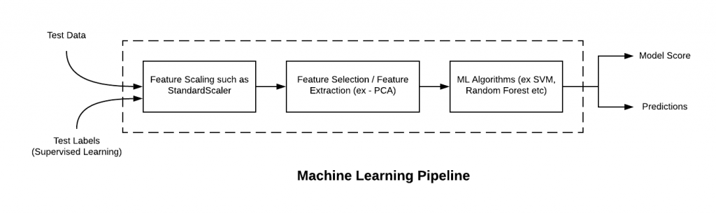
What does this mean? In practice this means that you can use all the regression and classification models shown in the figure below in the same way, they will all have a fit() method that accepts X and y and a predict method that accepts X and returns the predictions.

The estimator objects can be always used in the same way

Using these objects, instead of the mean directly, allows you to easily swap them with other models in pipelines, where one chains many data transformation steps (see section 6).
4.1. Build dummy models
$\color{DarkBlue}{\textsf{Short Question}}$
- If you call
.fit(X, y)on aDummyRegressordoes it actually use theX? If not, why is there still the place for theXin the function? If yes, how does it use it?
$\color{DarkBlue}{\textsf{Short Exercise}}$
- Create
DummyRegressorinstances formean,median. (e.g.dummyinstance = DummyRegressor(strategy='mean')) - Train them on the training data (
dummyinstance.fit(df_train[FEATURES], df_train[TARGET]))
Click here for hints
- to create
DummyRegressoryou can for example usedummyregressor_mean = DummyRegressor(strategy='mean') - to see the implementation of the
DummyRegressoryou can check out the source code on GitHub
# Build DummyRegressors
dummyregressor_mean = DummyRegressor(strategy='mean')
dummyregressor_median = DummyRegressor(#fillme)
# Fit Dummy Regressors
dummyregressor_mean.fit(df_train_stratified[FEATURES], df_train_stratified[TARGET])
dummyregressor_median.fit(#fillme)
Evaluate the performance of the dummy models
$\color{DarkBlue}{\textsf{Short Exercise}}$
- Calculate maximum error, mean absolute error and mean square error for the dummy regressors on training and test set. What would you expect those numbers to be?
- Do the actual values surprise you?
- What does this mean in practice for reporting of metrics/the reasoning behind using baseline models
It can be handy to store our metrics of choice in a nested dictionary (Python dictionaries are key-value pairs):
{
    'dummyestimator1': {
                        'metric_a_key': metric_a_value,
                        'metric_b_key': metric_b_value
                    },
    'dummyestimator2': {
                        'metric_a_key': metric_a_value,
                        'metric_b_key': metric_b_value
                    },
 }
You will now write functions get_regression_metrics(model, X, y_true) that compute the metrics and return this dictionary for a given model. The predict method takes the feature matrix $\mathbf{X}$ as input.
In them, we calculate
$\mathrm {MAE} =\frac{\sum _{i=1}^{n}\left|Y_{i}-\hat{y}_{i}\right|}{n}.$
and
$\mathrm {MSE} = {\frac {1}{n}}\sum _{i=1}^{n}(Y_{i}-{\hat {Y_{i}}})^{2}.$
where $\hat{y}$ are the predictions and, $Y_{i}$ the true values.
as well as the maximum error.
Click here for hints
- to perform a prediction using a estimator object, you can call
classifier.predict(X) - to calculate metrics, you can for example call
accuracy_score(true_values, predicted_values)
def get_regression_metrics(model, X, y_true):
    """
    Get a dicionary with regression metrics:

    model: sklearn model with predict method
    X: feature matrix
    y_true: ground truth labels
    """
    y_predicted = model.predict(#fillme)

    mae = mean_absolute_error(#fillme)
    mse = mean_squared_error(#fillme)
    maximum_error = max_error(#fillme)

    metrics_dict = {
        'mae': mae,
        'mse': mse,
        'max_error': maximum_error
    }

    return metrics_dict
dummy_regressors = [
    ('mean', dummyregressor_mean),
    ('median', dummyregressor_median)
]
dummy_regressor_results_test = {} # initialize empty dictionary
dummy_regressor_results_train = {}

# loop over the dummy_regressor list
# if you have a tuple regressorname, regressor = (a, b) that is automatically expanded into the variables
# a = regressorname, b = regressor
for regressorname, regressor in dummy_regressors:
    print(f"Calculating metrics for {regressorname}")
    dummy_regressor_results_test[regressorname] = get_regression_metrics(#fillme)
    dummy_regressor_results_train[regressorname] = get_regression_metrics(#fillme)
5. Build actual regression models
Let's build a simple kernel ridge regression (KRR) machine learning model and train it with our raw data. You can try different kernels, but we recommend to start with the Gaussian radial basis function ('rbf') kernel.
$\color{DarkBlue}{\textsf{Short Question}}$
- Do you expect this model to perform better than the dummy models?
- Train it and then calculate the performance metrics on the training and test set. How do they compare to the performance of the dummy models?
- What is the shape of the Kernel and of the weights? (you can check your answer by looking at the
dual_coef_attribute of the KRR instance. You can get shapes of objects using theshapeatrribute
# Train the model with a Gaussian kernel
krr = KernelRidge(kernel='rbf')
krr.fit(#fillme)
# get the metrics on the train and the test set using the get_regression_metrics functions (as above)
6. Evaluate the model performance in detail
We have trained our first machine learning model! We'll first have a closer look at its performance, before learning how to improve it.
$\color{DarkBlue}{\textsf{Short Exercise}}$
- Create a parity plot (true values against predictions)for the training and test data
- Plot a histogram of the distribution of the training and test errors on the training and test set. Plot the errors also as a function of the true value
- Let's assume we would like to use our model for pre-screening a library of millions of porous materials to zoom-in on those with the most promising gas uptake. Could you tolerate the errors of your model?
- Compare the parity plots for this model with the ones for the dummy models.
Use the plotting functions below the evaluate all the following models you train.
For this exercise, it can be handy to save the results in a dictionary, e.g.
(python)
res_train = {
    'y true': [],
    'y pred': []
}
Click here for hints for plotting
- If you want to use matplotlib to make the parity plots, you can use the hist2d function
- To create the frequencies and the edges of a histogram, one can use
np.histogram
# Create dictionaries with training and test results to create parity plots
res_train = {
    'y true': # fillme using the dataframe,
    'y pred': # fillme using the model prediction
}

res_test = {
    'y true': # fillme using the dataframe
    'y pred': # fillme using the model prediction
}
Now, lets calculate the errors
res_train["error"] = res_train["y true"] - res_train["y pred"]
res_test["error"] = res_test["y true"] - res_test["y pred"]
Now, plot the parity plots and error distributions
Click here for hints for plotting
If you want interactive plots, you can use the following code:
hv.extension("bokeh")
hex_train = hv.HexTiles(res_train, ["y true", "y pred"]).hist(
    dimension=["y true", "y pred"]
)
hex_test = hv.HexTiles(res_test, ["y true", "y pred"]).hist(
    dimension=["y true", "y pred"]
)
hex_train + hex_test
# plot it
hist_density(res_train['y true'], res_train['y pred'], xlabel='y true', ylabel='y pred', title='Train')
hist_density(res_test['y true'], res_test['y pred'], xlabel='y true', ylabel='y pred', title='Test')
7. Improve the model
Our training set still has a couple of issues you might have noticed:
- The feature values are not scaled (different features are measured in different units ...)
- Some features are basically constant, i.e. do not contain relevant information and just increase the dimensionality of the problem
- Some feature distributions are skewed (which is more relevant for some models than for others ...)
$\color{DarkBlue}{\textsf{Short Question}}$
- Why might the scaling of the features be relevant for a machine learning model?
7.1. Standard scaling and building a first pipeline
Given that we will now go beyond training a single model, we will build Pipelines, which are objects that can collect a selection of transformations and estimators. This makes it quite easy to apply the same set of operations to different datasets. A simple pipeline might be built as follows
$\color{DarkBlue}{\textsf{Short Exercise}}$
- Build a pipline that first performs standard scaling and then fits a KRR. Call it
pipe_w_scaling. - Fit it on the training set
- Make predictions, calculate the errors and make the parity plots
Click here for hints
- the
fit,predictmethods also work for pipelines
pipe_w_scaling = Pipeline(
   [
       ('scaling', StandardScaler()),
       ('krr', #fillme)
   ]
)
7.2. Hyperparameter optimization
A key component we did not optimize so far are hyperparameters. Those are parameters of the model that we usually cannot learn from the data but have to fix before we train the model. Since we cannot learn those parameters it is not trivial to select them. Hence, what we typically do in practice is to create another set, a "validation set", and use it to test models trained with different hyperparameters.
The most common approach to hyperparameter optimization is to define a grid of all relevant parameters and to search over the grid for the best model performance.
$\color{DarkBlue}{\textsf{Short Exercise}}$
- Think about which parameters you could optimize in the pipeline. Note that your KRR model has two parameters you can optimize. You can also switch off some steps by setting them to `None'.
- For each parameter you need to define a resonable grid to search over.
- Recall, what k-fold cross-validation does. Run the hyperparameter optimization using 5-fold cross-validation (you can adjust the number of folds according to your computational resources/impatience. It turns out at k=10 is the best tradeoff between variance and bias).
Tune the hyperparameters until you are statisfied (e.g., until you cannot improve the cross validated error any more)
- Why don't we use the test set for hyperparameter tuning but instead test on the validation set?
- Evaluate the model performance by calculating the performance metrics (MAE, MSE, max error) on the training and the test set.
- Optional: Instead of grid search, try to use random search on the same grid (
RandomizedSearchCV) and fix the number of evaluations (n_iter) to a fraction of the number of evaluations of grid search. What do you observe and conclude?
$\color{DarkRed}{\textsf{Tips}}$
If you want to see what is happening, set the
verbosityargument of theGridSearchCVobject to a higher number.If you want to speed up the optimization, you can run it in parallel by setting the
n_jobsargument to the number of workers. If you set it to -1 it will use all available cores. Using all cores might freeze your computer if you do not have enough memoryIf the optimization is too slow, reduce the number of data points in your set, the number of folds or the grid size. Note that it can also be a feasible strategy to first use a coarser grid and the a finer grid for fine-tuning.
For grid search, you need to define a parameter grid, which is a dictionary of the following form:
(python)
param_grid = {
                    'pipelinestage__parameter': np.logspace(-4,1,10),
                    'pipelinestage': [None, TransformerA(), TransformerB()]
            }
After the search, you can access the best model with
.best_estimator_and the best parameters with.best_params_on the GridSearchCV instance. For examplegrid_krr.best_estimator_If you initialize the GridSearchCV instance with
refit=Trueit will automatically train the model with all training data (and not only the training folds from cross-validations)
The double underscore (dunder) notation works recursively and specifies the parameters for any pipeline stage.
For example, ovasvm__estimator__cls__C would specifiy the C parameter of the estimator in the one-versus-rest classifier ovasvm.
You can print all parameters of the pipeline using print(sorted(pipeline.get_params().keys()))
Click here for hints about pipelines and grid search
- You can use the
np.logspacefunction to generate a grid for values that you want to vary on a logarithmic scale - There are two hyperparameters for KRR: the regularization strength
alphaand the Gaussian widthgamma - For the regularization strength, values between 1 and 1e-3 can be reasonable. For gamma you can use the median heuristic, gamma = 1 / median, or values between 1e-3 and 1e3
# Define the parameter grid and the grid search object
param_grid = {
                    'scaling': [MinMaxScaler(), StandardScaler()], # test different scaling methods
                    'krr__alpha': #fillme,
                    'krr__#fillme': #fillme
            }

grid_krr = GridSearchCV(#your pipeline, param_grid=param_grid,
                        cv=#number of folds, verbose=2, n_jobs=2)

# optional random search
#random_krr = RandomizedSearchCV(#your pipeline, param_distributions=param_grid, n_iter=#number of evaluations,
#                        cv=#number of folds, verbose=2, n_jobs=2
)
# run the grid search by calling the fit method
grid_krr.fit(#fillme)
# optional random search
# random_krr.fit(#fillme)
# get the performance metrics
get_regression_metrics(#fillme)
Click here for some more information about hyperparameter optimization
Grid search is not the most efficient way to perform hyperparamter optimization. Even random search was shown to be more efficient. Really efficient though are Bayesian optimization approaches like TPE. This is implemented in the hyperopt library, which is also installed in your conda environment.Click here for hyperparameter optimization with hyperopt (advanded and optional outlook)
Import the tools we need
from hyperopt import fmin, tpe, hp, STATUS_OK, Trials, mix, rand, anneal, space_eval
from functools import partial
Define the grid
param_hyperopt = {
    "krr__alpha": hp.loguniform("krr__alpha", np.log(0.001), np.log(10)),
    "krr__gamma": hp.loguniform("krr__gamma", np.log(0.001), np.log(10)),
}
Define the objective function
def objective_function(params):
    pipe.set_params(
        **{
            "krr__alpha": params["krr__alpha"],
            "krr__gamma": params["krr__gamma"],
        }
    )
    score = cross_val_score(
        pipe, X_train, y_train, cv=10, scoring="neg_mean_absolute_error"
    ).mean()
    return {"loss": -score, "status": STATUS_OK}
We will use a search in which we mix random search, annealing and tpe
trials = Trials()
mix_search = partial(
   mix.suggest,
   p_suggest=[(0.15, rand.suggest), (0.15, anneal.suggest), (0.7, tpe.suggest)],
)
Now, we can minimize the objective function.
best_param = fmin(
        objective_function,
        param_hyperopt,
        algo=mix_search,
        max_evals=MAX_EVALES,
        trials=trials,
        rstate=np.random.RandomState(RANDOM_SEED),
    )
8. Feature Engineering
Finally, we would like to remove features with low variance. This can be done by setting a variance threshold.
$\color{DarkBlue}{\textsf{Short Question}}$
- What is the reasoning behind doing this?
- When might it go wrong and why?
$\color{DarkBlue}{\textsf{Short Exercise}}$
- Add a variance threshold to the pipeline (select the correct function argument)
- Use random search for hyperparameter optimization, retrain the pipeline, and calculate the performance metrics (max error, MAE, MSE) on the training and test set
- If you could improve the predictive performance, do not forget to also run the model for the Kaggle competition!
# Define the pipeline
pipe_variance_threshold = Pipeline(
    # fillme with the pipeline steps
    [
        ('variance_treshold', VarianceThreshold(#fillme with threshold)),
        #fillme with remaining pipeline steps
    ]
)
param_grid_variance_threshold = {
                    'scaling': [None, StandardScaler()],
                    'krr__alpha': #fillme,
                    'krr__#fillme': #fillme,
                    'variance_treshold__threshold': #fillme
            }

random_variance_treshold = RandomizedSearchCV(#your pipeline, param_distributions=param_grid, n_iter=#number of evaluations,
                        cv=#number of folds, verbose=2, n_jobs=2)
# Fit the pipeline and run the evaluation
random_variance_treshold.fit(#fillme)
$\color{DarkBlue}{\textsf{Short Exercise (optional)}}$
- replace the variance threshold with a model-based feature selection
('feature_selection', SelectFromModel(LinearSVC(penalty="l1"))) or any feature selection method that you would like to try
9. Saving the model
Now, that we spent so much time in optimizing our model, we do not want to loose it.
$\color{DarkBlue}{\textsf{Short Exercise}}$
- use the joblib library to save your model
- make sure you can load it again
# Dump your model
joblib.dump(model, filename)
# Try to load it again
model_loaded = joblib.load(filename)
10. Influence of Regularization
$\color{DarkBlue}{\textsf{Short Exercise}}$
- what happens if you set $\alpha$ to a really small or to large value? Why is this the case explain what the parameter means using the equation derived in the lectures?
To test this, fix this value in one of your pipelines, retrain the models (re-optimizing the other hyperparameters) and rerun the performance evaluation.
Click here for hints
- Check the derivation for ridge regression and KRR in the notes.
- Also remember the loss landscapes we discussed in the lectures about LASSO.
11. Interpreting the model
Now, that our model performs decently, we would like to know which features are mainly responsible for this, i.e. how the model performs its reasoning.
One method to do so is the permutation feature importance technique.
$\color{DarkBlue}{\textsf{Short question}}$
We use both descriptors that encode the pore geometry (density, pore diameters, surface areas) as well as some that describe the chemistry of the MOF (the RACs).
- Would you expect the relative importance of these features to be different for prediction of gas adsorption at high vs low gas pressure?
Click here for a hint
- An article from Diego et al. (10.1021/acs.chemmater.8b02257) gives some hints.
$\color{DarkBlue}{\textsf{Short Exercise}}$
- Complete the function
_calculate_permutation_scores(which we took from thesklearnpackage) and which is needed to calculate the permutation feature importance using thepermutation_importancefunction.
def _calculate_permutation_scores(estimator, X, y, col_idx, random_state,
                                  n_repeats, scorer):
    """Calculate score when `col_idx` is permuted. Based on the sklearn implementation

    estimator: sklearn estimator object
    X: pd.Dataframe or np.array
    y: pd.Dataframe or np.array
    col_idx: int
    random_state: int
    n_repeats: int
    scorer: function that takes model, X and y_true as arguments
    """
    random_state = check_random_state(random_state)

    X_permuted = X.copy()
    scores = np.zeros(n_repeats)
    # get the indices
    shuffling_idx = np.arange(X.shape[0])
    for n_round in range(n_repeats):
        # FILL BELOW HERE
        # shuffle them (fill in what you want to shuffle)
        random_state.shuffle(#fillme)

        # Deal with dataframes
        if hasattr(X_permuted, "iloc"):
            # .iloc selects the indices from a dataframe and you give it [row, column]
            col = X_permuted.iloc[shuffling_idx, col_idx]
            col.index = X_permuted.index
            X_permuted.iloc[:, col_idx] = col

        # Deal with numpy arrays
        else:
            # FILL BELOW HERE
            # array indexing is [row, column]
            X_permuted[:, col_idx] = X_permuted[#fillme]

        # Get the scores
        feature_score = scorer(estimator, X_permuted, y)

        # record the scores in array
        scores[n_round] = feature_score

    return scores
Nothing to change in the function below, it just call the _calculate_permutation_scores function you just completed.
def permutation_importance(
    estimator,
    X,
    y,
    scoring="neg_mean_absolute_error",
    n_repeats=5,
    n_jobs=2,
    random_state=None,
):
    """Permutation importance for feature evaluation
    estimator : object
        An estimator that has already been :term:`fitted` and is compatible
        with :term:`scorer`.
    X : ndarray or DataFrame, shape (n_samples, n_features)
        Data on which permutation importance will be computed.
    y : array-like or None, shape (n_samples, ) or (n_samples, n_classes)
        Targets for supervised or `None` for unsupervised.
    scoring : string, callable or None, default=None
        Scorer to use. It can be a single
        string (see :ref:`scoring_parameter`) or a callable (see
        :ref:`scoring`). If None, the estimator's default scorer is used.
    n_repeats : int, default=5
        Number of times to permute a feature.
    n_jobs : int or None, default=2
        The number of jobs to use for the computation.
        `None` means 1 unless in a :obj:`joblib.parallel_backend` context.
        `-1` means using all processors. See :term:`Glossary <n_jobs>`
        for more details.
    random_state : int, RandomState instance, or None, default=None
        Pseudo-random number generator to control the permutations of each
        feature. See :term:`random_state`.
    """
    # Deal with dataframes
    if not hasattr(X, "iloc"):
        X = check_array(X, force_all_finite="allow-nan", dtype=None)

    # Precompute random seed from the random state to be used
    # to get a fresh independent RandomState instance for each
    # parallel call to _calculate_permutation_scores, irrespective of
    # the fact that variables are shared or not depending on the active
    # joblib backend (sequential, thread-based or process-based).
    random_state = check_random_state(random_state)
    random_seed = random_state.randint(np.iinfo(np.int32).max + 1)

    # Determine scorer from user options.
    scorer = check_scoring(estimator, scoring=scoring)
    # get the performance score on the unpermuted data
    baseline_score = scorer(estimator, X, y)

    # run the permuted evaluations in parallel for each column
    scores = Parallel(n_jobs=n_jobs)(
        delayed(_calculate_permutation_scores)(
            estimator, X, y, col_idx, random_seed, n_repeats, scorer
        )
        for col_idx in range(X.shape[1])
    )

    # get difference two
    importances = baseline_score - np.array(scores)

    # return the results (dictionary)
    return Bunch(
        importances_mean=np.mean(importances, axis=1),
        importances_std=np.std(importances, axis=1),
        importances=importances,
    )
$\color{DarkBlue}{\textsf{Short Exercise}}$
- Use your function to find the five most important features.
- Which are they? Did you expect this result?
permutation_results = permutation_importance(#fillme)
permutation_results["features"] = FEATURES
bars = hv.Bars(
    permutation_results, "features", ["importances_mean", "importances_std"]
).sort("importances_mean", reverse=True)
errors = hv.ErrorBars(
    permutation_results, "features", vdims=["importances_mean", "importances_std"]
).sort("importances_mean", reverse=True)

bars * errors
Click here for hints
- To get the top
n indices of an arraya, you can usenp.argsort(a)[-n:] - Get the feature names from the
FEATURESlist - combined this might look like
np.array(FEATURES)[np.argsort(a)[-n:]]
Click here for more information on model interpretation
The permutation feature importance technique is not a silver bullet, e.g. there are issues with correlated features. However, it is likely a better choice than feature importance, like impurity decrease, derived from random forests).12. Submit your best model to Kaggle
Join the Kaggle competition for this course! For this you can:
- try to continue optimizing your KRR model
- try to use a new model (browse the sklearn documentation for ideas or check out xgboost
The important parts for us here are:
- that you make an attempt to improve your model, discuss this attempt, and use proper models to measure potential improvement
- we will not grade you based on how "fancy" or model is or how well it performs but rather on whether you do something reasonable that is well motivated in your discussion
- you do not need to try both a model and continue optimizing your model. Doing one of them is, in principle, "enough"
Use then your best model to create a submission.csv with your predictions to join the competition and upload it to the competition site.
kaggle_data = pd.read_csv('data/features.csv')
kaggle_predictions = #fillme.predict(kaggle_data[FEATURES])
submission = pd.DataFrame({"id": kaggle_data["id"], "prediction": kaggle_predictions})

submission.to_csv("submission.csv", index=False)