Theory
Ideally, spatial channels should be independent to each other, i.e. uncorrelated.
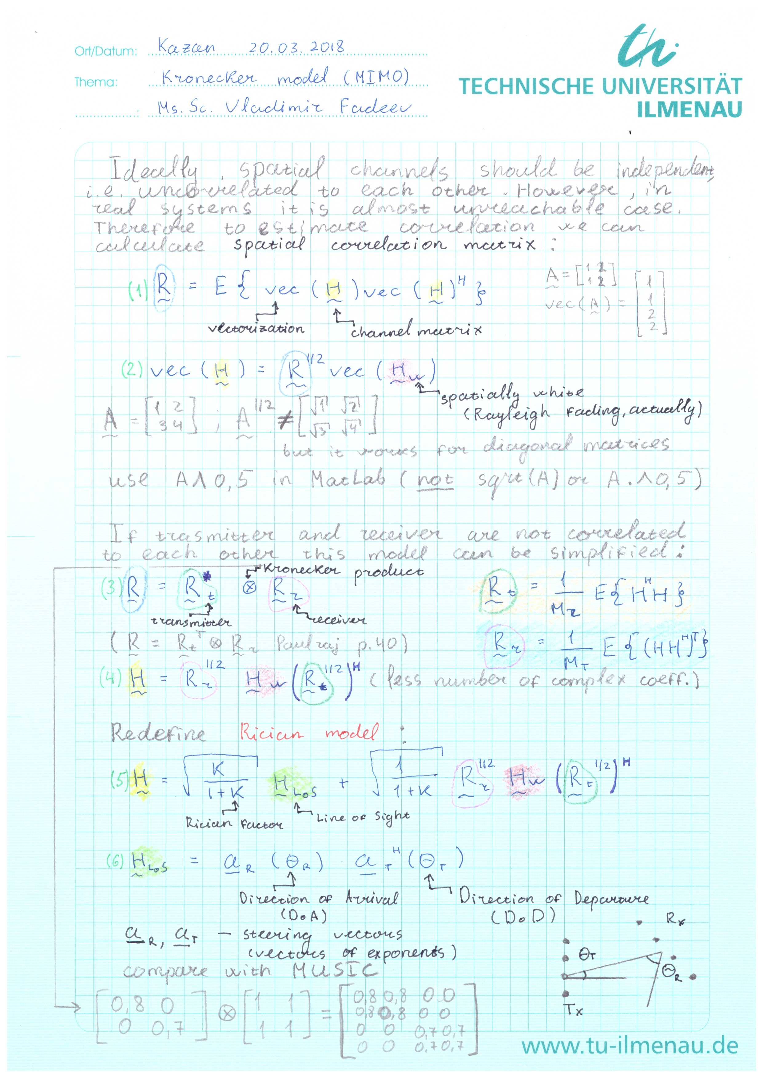
However, it is almost unreachable case in real systems. Therefore we can calculate spatial correlation matrix to estimate correlation:
$$ \mathbf{R} = E\left\{vec\left(H\right)\left(vec\left(H\right)\right)^H\right\} \qquad (1) $$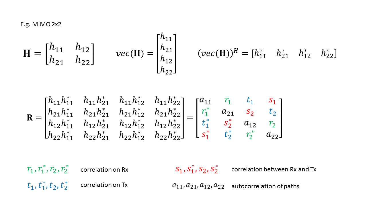
If the Tx and Rx sides are uncorrelated (e.g. fig. 1) to each other, simplification can be applied: Kronecker model.

Fig. 1. The scatters model in case of uncorrelated Rx and Tx. Green dots mean scatters, blue and red - RX and Tx.
However, in case of correlated channel (e.g. fig. 2) the formula (1) should be used.
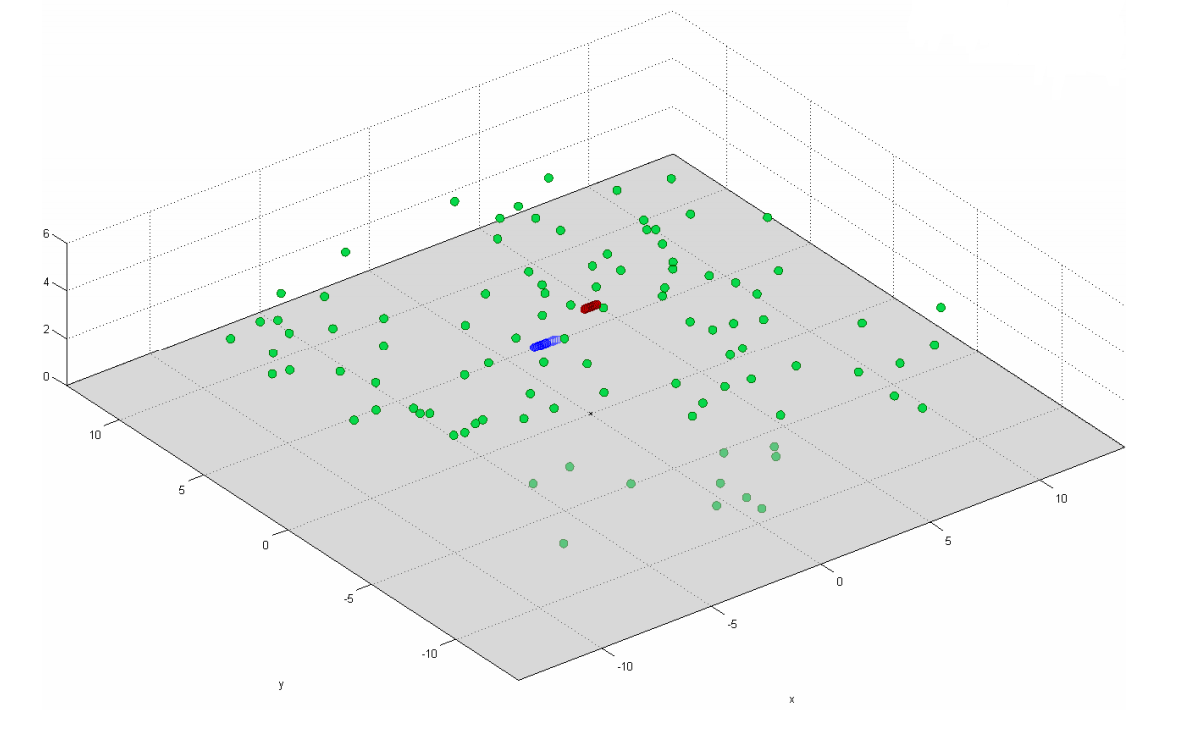
Fig. 2. The scatters model in case of correlated Rx and Tx. Green dots mean scatters, blue and red - RX and Tx.
Tasks
Task #1
If we consider the Kroneker model, can we say that $r_1 = r_2$ and $t_1 = t_2$?
What about $3\times 3$ or $4 \times 3$ channels?
Hint: See [1, p.40] about the Kronecker product and properties of $\mathbf{R}_T$ and $\mathbf{R}_R$.
Task #2
Calculate all of the $\gamma^{opt}$ if $\mathbf{R}_T = \begin{bmatrix} 0.6 & 0 \\ 0 & 0.7 \end{bmatrix}$ and $\mathbf{R}_R = \begin{bmatrix} 1 && 1 \\ 1 && 1 \end{bmatrix}$, if SNR $-> + \infty$ (values of co-variance matrices are random, the main part is the logic of the solution).
Hint: Use the Water-pouring algorithm and see [1, p.40].
Task #3
Is it possible to use Kronecker model for the following case: $$\mathbf{R} = \begin{bmatrix} 1 && 0.6 && 0.4 && 0.9 \\ 0.6 && 1 && 0.8 && 0.4 \\ 0.4 && 0.8 && 1 && 0.6 \\ 0.9 && 0.4 && 0.6 && 1 \end{bmatrix}$$
Explain why, if not. If yes, explain too.
Reference
- Paulraj, Arogyaswami, Rohit Nabar, and Dhananjay Gore. Introduction to space-time wireless communications. Cambridge university press, 2003.