Deep Learning for Movie Recommendation
In this notebook, I'll build a deep learning model movie recommendations system on the MovieLens 1M dataset.
This will be my 3rd attempt doing this.
- In the 1st attempt, I tried out content-based and memory-based collaboratice filtering, which rely on the calculation of users and movies' similarity scores. As no training or optimization is involved, these are easy to use approaches. But their performance decrease when we have sparse data which hinders scalability of these approaches for most of the real-world problems.
- In the 2nd attempt, I tried out a matrix factorization model-based collaborative filtering approach called Singular Vector Decomposition, which reduces the dimension of the dataset and gives low-rank approximation of user tastes and preferences.
In this post, I will use a Deep Learning / Neural Network approach that is up and coming with recent development in machine learning and AI technologies.

Loading Datasets
Similar to what I did for the previous notebooks, I loaded the 3 datasets into 3 dataframes: ratings, users, and movies. Additionally, to make it easy to use series from the ratings dataframe as training inputs and output to the Keras model, I set max_userid as the max value of user_id in the ratings and max_movieid as the max value of movie_id in the ratings.
# Import libraries
%matplotlib inline
import math
import numpy as np
import pandas as pd
import matplotlib.pyplot as plt

# Reading ratings file
ratings = pd.read_csv('ratings.csv', sep='\t', encoding='latin-1',
                      usecols=['user_id', 'movie_id', 'user_emb_id', 'movie_emb_id', 'rating'])
max_userid = ratings['user_id'].drop_duplicates().max()
max_movieid = ratings['movie_id'].drop_duplicates().max()

# Reading ratings file
users = pd.read_csv('users.csv', sep='\t', encoding='latin-1',
                    usecols=['user_id', 'gender', 'zipcode', 'age_desc', 'occ_desc'])

# Reading ratings file
movies = pd.read_csv('movies.csv', sep='\t', encoding='latin-1',
                     usecols=['movie_id', 'title', 'genres'])
Matrix Factorization for Collaborative Filtering
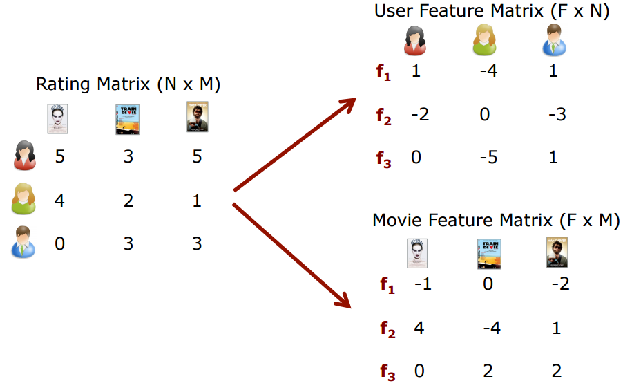
I have discussed this extensively in my 2nd notebook, but want to revisit it here as the baseline approach. The idea behind matrix factorization models is that attitudes or preferences of a user can be determined by a small number of hidden factors. We can call these factors as Embeddings.
Intuitively, we can understand embeddings as low dimensional hidden factors for movies and users. For e.g. say we have 3 dimensional embeddings for both movies and users.
For instance, for movie A, the 3 numbers in the movie embedding matrix represent 3 different characteristics about the movie, such as:
- How recent is the movie A?
- How much special effects are in movie A?
- How CGI-driven is movie A?
For user B, the 3 numbers in the user embedding matrix represent:
- How much does user B like Drama movie?
- How likely does user B to give a 5-star rating?
- How often does user B watch movies?
I definitely would want to create a training and validation set and optimize the number of embeddings by minimizing the RMSE. Intuitively, the RMSE will decrease on the training set as the number of embeddings increases (because I'm approximating the original ratings matrix with a higher rank matrix). Here I create a training set by shuffling randomly the values from the original ratings dataset.
# Create training set
shuffled_ratings = ratings.sample(frac=1., random_state=RNG_SEED)

# Shuffling users
Users = shuffled_ratings['user_emb_id'].values
print 'Users:', Users, ', shape =', Users.shape

# Shuffling movies
Movies = shuffled_ratings['movie_emb_id'].values
print 'Movies:', Movies, ', shape =', Movies.shape

# Shuffling ratings
Ratings = shuffled_ratings['rating'].values
print 'Ratings:', Ratings, ', shape =', Ratings.shape
Users: [1284 1682 2367 ... 2937 2076 4665] , shape = (1000209,)
Movies: [1093 3071   44 ... 1135 1731 1953] , shape = (1000209,)
Ratings: [4 5 4 ... 5 5 1] , shape = (1000209,)
Deep Learning Model
The idea of using deep learning is similar to that of Model-Based Matrix Factorization. In matrix factorizaion, we decompose our original sparse matrix into product of 2 low rank orthogonal matrices. For deep learning implementation, we don’t need them to be orthogonal, we want our model to learn the values of embedding matrix itself. The user latent features and movie latent features are looked up from the embedding matrices for specific movie-user combination. These are the input values for further linear and non-linear layers. We can pass this input to multiple relu, linear or sigmoid layers and learn the corresponding weights by any optimization algorithm (Adam, SGD, etc.).
Build the Model
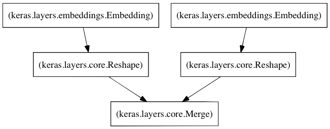
I created a sparse matrix factoring algorithm in Keras for my model in CFModel.py. Here are the main components:
- A left embedding layer that creates a Users by Latent Factors matrix.
- A right embedding layer that creates a Movies by Latent Factors matrix.
- When the input to these layers are (i) a user id and (ii) a movie id, they'll return the latent factor vectors for the user and the movie, respectively.
- A merge layer that takes the dot product of these two latent vectors to return the predicted rating.
This code is based on the approach outlined in Alkahest's blog post Collaborative Filtering in Keras.
# Import Keras libraries
from keras.callbacks import Callback, EarlyStopping, ModelCheckpoint
# Import CF Model Architecture
from CFModel import CFModel
/Users/khanhnamle/anaconda2/lib/python2.7/site-packages/h5py/__init__.py:34: FutureWarning: Conversion of the second argument of issubdtype from `float` to `np.floating` is deprecated. In future, it will be treated as `np.float64 == np.dtype(float).type`.
  from ._conv import register_converters as _register_converters
Using TensorFlow backend.
# Define constants
K_FACTORS = 100 # The number of dimensional embeddings for movies and users
TEST_USER = 2000 # A random test user (user_id = 2000)
I then compile the model using Mean Squared Error (MSE) as the loss function and the AdaMax learning algorithm.
# Define model
model = CFModel(max_userid, max_movieid, K_FACTORS)
# Compile the model using MSE as the loss function and the AdaMax learning algorithm
model.compile(loss='mse', optimizer='adamax')
CFModel.py:28: UserWarning: The `Merge` layer is deprecated and will be removed after 08/2017. Use instead layers from `keras.layers.merge`, e.g. `add`, `concatenate`, etc.
  self.add(Merge([P, Q], mode='dot', dot_axes=1))
Train the Model
Now I need to train the model. This step will be the most-time consuming one. In my particular case, for our dataset with nearly 1 million ratings, almost 6,000 users and 4,000 movies, I trained the model in roughly 6 minutes per epoch (30 epochs ~ 3 hours) inside my Macbook Laptop CPU. I spitted the training and validataion data with ratio of 90/10.
# Callbacks monitor the validation loss
# Save the model weights each time the validation loss has improved
callbacks = [EarlyStopping('val_loss', patience=2),
             ModelCheckpoint('weights.h5', save_best_only=True)]

# Use 30 epochs, 90% training data, 10% validation data
history = model.fit([Users, Movies], Ratings, nb_epoch=30, validation_split=.1, verbose=2, callbacks=callbacks)
/Users/khanhnamle/anaconda2/lib/python2.7/site-packages/keras/models.py:944: UserWarning: The `nb_epoch` argument in `fit` has been renamed `epochs`.
  warnings.warn('The `nb_epoch` argument in `fit` '
Train on 900188 samples, validate on 100021 samples
Epoch 1/30
 - 387s - loss: 8.2727 - val_loss: 2.2829
Epoch 2/30
 - 316s - loss: 1.4957 - val_loss: 1.1248
Epoch 3/30
 - 319s - loss: 1.0059 - val_loss: 0.9370
Epoch 4/30
 - 317s - loss: 0.8957 - val_loss: 0.8764
Epoch 5/30
 - 316s - loss: 0.8495 - val_loss: 0.8461
Epoch 6/30
 - 355s - loss: 0.8182 - val_loss: 0.8228
Epoch 7/30
 - 395s - loss: 0.7921 - val_loss: 0.8045
Epoch 8/30
 - 395s - loss: 0.7695 - val_loss: 0.7921
Epoch 9/30
 - 394s - loss: 0.7477 - val_loss: 0.7807
Epoch 10/30
 - 406s - loss: 0.7269 - val_loss: 0.7700
Epoch 11/30
 - 371s - loss: 0.7060 - val_loss: 0.7614
Epoch 12/30
 - 332s - loss: 0.6849 - val_loss: 0.7543
Epoch 13/30
 - 319s - loss: 0.6639 - val_loss: 0.7483
Epoch 14/30
 - 340s - loss: 0.6428 - val_loss: 0.7458
Epoch 15/30
 - 358s - loss: 0.6218 - val_loss: 0.7428
Epoch 16/30
 - 315s - loss: 0.6009 - val_loss: 0.7433
Epoch 17/30
 - 314s - loss: 0.5801 - val_loss: 0.7424
Epoch 18/30
 - 314s - loss: 0.5596 - val_loss: 0.7458
Epoch 19/30
 - 313s - loss: 0.5396 - val_loss: 0.7481
Root Mean Square Error
During the training process above, I saved the model weights each time the validation loss has improved. Thus, I can use that value to calculate the best validation Root Mean Square Error.
# Show the best validation RMSE
min_val_loss, idx = min((val, idx) for (idx, val) in enumerate(history.history['val_loss']))
print 'Minimum RMSE at epoch', '{:d}'.format(idx+1), '=', '{:.4f}'.format(math.sqrt(min_val_loss))
Minimum RMSE at epoch 17 = 0.8616
The best validation loss is 0.7424 at epoch 17. Taking the square root of that number, I got the RMSE value of 0.8616, which is better than the RMSE from the SVD Model (0.8736).
Predict the Ratings
The next step is to actually predict the ratings a random user will give to a random movie. Below I apply the freshly trained deep learning model for all the users and all the movies, using 100 dimensional embeddings for each of them. I also load pre-trained weights from weights.h5 for the model.
# Use the pre-trained model
trained_model = CFModel(max_userid, max_movieid, K_FACTORS)
# Load weights
trained_model.load_weights('weights.h5')
As mentioned above, my random test user is has ID 2000.
# Pick a random test user
users[users['user_id'] == TEST_USER]
| user_id | gender | zipcode | age_desc | occ_desc | |
|---|---|---|---|---|---|
| 1999 | 2000 | M | 44685 | 18-24 | college/grad student |
Here I define the function to predict user's rating of unrated items, using the rate function inside the CFModel class in CFModel.py.
# Function to predict the ratings given User ID and Movie ID
def predict_rating(user_id, movie_id):
    return trained_model.rate(user_id - 1, movie_id - 1)
Here I show the top 20 movies that user 2000 has already rated, including the predictions column showing the values that used 2000 would have rated based on the newly defined predict_rating function.
user_ratings = ratings[ratings['user_id'] == TEST_USER][['user_id', 'movie_id', 'rating']]
user_ratings['prediction'] = user_ratings.apply(lambda x: predict_rating(TEST_USER, x['movie_id']), axis=1)
user_ratings.sort_values(by='rating',
                         ascending=False).merge(movies,
                                                on='movie_id',
                                                how='inner',
                                                suffixes=['_u', '_m']).head(20)
| user_id | movie_id | rating | prediction | title | genres | |
|---|---|---|---|---|---|---|
| 0 | 2000 | 1639 | 5 | 3.724665 | Chasing Amy (1997) | Drama|Romance |
| 1 | 2000 | 2529 | 5 | 3.803218 | Planet of the Apes (1968) | Action|Sci-Fi |
| 2 | 2000 | 1136 | 5 | 4.495121 | Monty Python and the Holy Grail (1974) | Comedy |
| 3 | 2000 | 2321 | 5 | 4.010493 | Pleasantville (1998) | Comedy |
| 4 | 2000 | 2858 | 5 | 4.253924 | American Beauty (1999) | Comedy|Drama |
| 5 | 2000 | 2501 | 5 | 4.206387 | October Sky (1999) | Drama |
| 6 | 2000 | 2804 | 5 | 4.353670 | Christmas Story, A (1983) | Comedy|Drama |
| 7 | 2000 | 1688 | 5 | 3.710508 | Anastasia (1997) | Animation|Children's|Musical |
| 8 | 2000 | 1653 | 5 | 4.089375 | Gattaca (1997) | Drama|Sci-Fi|Thriller |
| 9 | 2000 | 527 | 5 | 5.046471 | Schindler's List (1993) | Drama|War |
| 10 | 2000 | 1619 | 5 | 3.688177 | Seven Years in Tibet (1997) | Drama|War |
| 11 | 2000 | 110 | 5 | 3.966857 | Braveheart (1995) | Action|Drama|War |
| 12 | 2000 | 1193 | 5 | 4.718451 | One Flew Over the Cuckoo's Nest (1975) | Drama |
| 13 | 2000 | 318 | 5 | 4.743262 | Shawshank Redemption, The (1994) | Drama |
| 14 | 2000 | 1748 | 5 | 3.779190 | Dark City (1998) | Film-Noir|Sci-Fi|Thriller |
| 15 | 2000 | 1923 | 5 | 3.264066 | There's Something About Mary (1998) | Comedy |
| 16 | 2000 | 1259 | 5 | 4.543493 | Stand by Me (1986) | Adventure|Comedy|Drama |
| 17 | 2000 | 595 | 5 | 4.334908 | Beauty and the Beast (1991) | Animation|Children's|Musical |
| 18 | 2000 | 2028 | 5 | 4.192429 | Saving Private Ryan (1998) | Action|Drama|War |
| 19 | 2000 | 1907 | 5 | 4.027490 | Mulan (1998) | Animation|Children's |
No surpise that these top movies all have 5-start rating. Some of the prediction values seem off (those with value 3.7, 3.8, 3.9 etc.).
Recommend Movies
Here I make a recommendation list of unrated 20 movies sorted by prediction value for user 2000. Let's see it.
recommendations = ratings[ratings['movie_id'].isin(user_ratings['movie_id']) == False][['movie_id']].drop_duplicates()
recommendations['prediction'] = recommendations.apply(lambda x: predict_rating(TEST_USER, x['movie_id']), axis=1)
recommendations.sort_values(by='prediction',
                          ascending=False).merge(movies,
                                                 on='movie_id',
                                                 how='inner',
                                                 suffixes=['_u', '_m']).head(20)
| movie_id | prediction | title | genres | |
|---|---|---|---|---|
| 0 | 953 | 4.868923 | It's a Wonderful Life (1946) | Drama |
| 1 | 668 | 4.866858 | Pather Panchali (1955) | Drama |
| 2 | 1423 | 4.859523 | Hearts and Minds (1996) | Drama |
| 3 | 3307 | 4.834415 | City Lights (1931) | Comedy|Drama|Romance |
| 4 | 649 | 4.802675 | Cold Fever (Á köldum klaka) (1994) | Comedy|Drama |
| 5 | 669 | 4.797451 | Aparajito (1956) | Drama |
| 6 | 326 | 4.784828 | To Live (Huozhe) (1994) | Drama |
| 7 | 3092 | 4.761148 | Chushingura (1962) | Drama |
| 8 | 3022 | 4.753003 | General, The (1927) | Comedy |
| 9 | 2351 | 4.720692 | Nights of Cabiria (Le Notti di Cabiria) (1957) | Drama |
| 10 | 926 | 4.719633 | All About Eve (1950) | Drama |
| 11 | 3306 | 4.718323 | Circus, The (1928) | Comedy |
| 12 | 3629 | 4.684521 | Gold Rush, The (1925) | Comedy |
| 13 | 3415 | 4.683432 | Mirror, The (Zerkalo) (1975) | Drama |
| 14 | 2609 | 4.678223 | King of Masks, The (Bian Lian) (1996) | Drama |
| 15 | 1178 | 4.674256 | Paths of Glory (1957) | Drama|War |
| 16 | 2203 | 4.656760 | Shadow of a Doubt (1943) | Film-Noir|Thriller |
| 17 | 954 | 4.654399 | Mr. Smith Goes to Washington (1939) | Drama |
| 18 | 3849 | 4.649190 | Spiral Staircase, The (1946) | Thriller |
| 19 | 602 | 4.645639 | Great Day in Harlem, A (1994) | Documentary |
Conclusion
In this notebook, I showed how to use a simple deep learning approach to build a recommendation engine for the MovieLens 1M dataset. This model performed better than all the approaches I attempted before (content-based, user-item similarity collaborative filtering, SVD). I can certainly improve this model's performance by making it deeper with more linear and non-linear layers. I leave that task to you then!