Linear Regression
Agenda
- Introducing the bikeshare dataset
- Reading in the data
- Visualizing the data
- Linear regression basics
- Form of linear regression
- Building a linear regression model
- Using the model for prediction
- Does the scale of the features matter?
- Working with multiple features
- Visualizing the data (part 2)
- Adding more features to the model
- Choosing between models
- Feature selection
- Evaluation metrics for regression problems
- Comparing models with train/test split and RMSE
- Comparing testing RMSE with null RMSE
- Creating features
- Handling categorical features
- Feature engineering
- Comparing linear regression with other models
Reading in the data
We'll be working with a dataset from Capital Bikeshare that was used in a Kaggle competition (data dictionary).
# read the data and set the datetime as the index
import pandas as pd
url = 'https://raw.githubusercontent.com/justmarkham/DAT8/master/data/bikeshare.csv'
bikes = pd.read_csv(url, index_col='datetime', parse_dates=True)
bikes.head()
| season | holiday | workingday | weather | temp | atemp | humidity | windspeed | casual | registered | count | |
|---|---|---|---|---|---|---|---|---|---|---|---|
| datetime | |||||||||||
| 2011-01-01 00:00:00 | 1 | 0 | 0 | 1 | 9.84 | 14.395 | 81 | 0 | 3 | 13 | 16 |
| 2011-01-01 01:00:00 | 1 | 0 | 0 | 1 | 9.02 | 13.635 | 80 | 0 | 8 | 32 | 40 |
| 2011-01-01 02:00:00 | 1 | 0 | 0 | 1 | 9.02 | 13.635 | 80 | 0 | 5 | 27 | 32 |
| 2011-01-01 03:00:00 | 1 | 0 | 0 | 1 | 9.84 | 14.395 | 75 | 0 | 3 | 10 | 13 |
| 2011-01-01 04:00:00 | 1 | 0 | 0 | 1 | 9.84 | 14.395 | 75 | 0 | 0 | 1 | 1 |
Questions:
- What does each observation represent?
- What is the response variable (as defined by Kaggle)?
- How many features are there?
# "count" is a method, so it's best to name that column something else
bikes.rename(columns={'count':'total'}, inplace=True)
Visualizing the data
import seaborn as sns
import matplotlib.pyplot as plt
%matplotlib inline
plt.rcParams['figure.figsize'] = (8, 6)
plt.rcParams['font.size'] = 14
# Pandas scatter plot
bikes.plot(kind='scatter', x='temp', y='total', alpha=0.2)
<matplotlib.axes._subplots.AxesSubplot at 0x18266cc0>

# Seaborn scatter plot with regression line
sns.lmplot(x='temp', y='total', data=bikes, aspect=1.5, scatter_kws={'alpha':0.2})
<seaborn.axisgrid.FacetGrid at 0x1867af28>

Form of linear regression
$y = \beta_0 + \beta_1x_1 + \beta_2x_2 + ... + \beta_nx_n$
- $y$ is the response
- $\beta_0$ is the intercept
- $\beta_1$ is the coefficient for $x_1$ (the first feature)
- $\beta_n$ is the coefficient for $x_n$ (the nth feature)
The $\beta$ values are called the model coefficients:
- These values are estimated (or "learned") during the model fitting process using the least squares criterion.
- Specifically, we are find the line (mathematically) which minimizes the sum of squared residuals (or "sum of squared errors").
- And once we've learned these coefficients, we can use the model to predict the response.
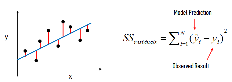
In the diagram above:
- The black dots are the observed values of x and y.
- The blue line is our least squares line.
- The red lines are the residuals, which are the vertical distances between the observed values and the least squares line.
Building a linear regression model
# create X and y
feature_cols = ['temp']
X = bikes[feature_cols]
y = bikes.total
# import, instantiate, fit
from sklearn.linear_model import LinearRegression
linreg = LinearRegression()
linreg.fit(X, y)
LinearRegression(copy_X=True, fit_intercept=True, n_jobs=1, normalize=False)
# print the coefficients
print linreg.intercept_
print linreg.coef_
6.04621295961
[ 9.17054048]
Interpreting the intercept ($\beta_0$):
- It is the value of $y$ when $x$=0.
- Thus, it is the estimated number of rentals when the temperature is 0 degrees Celsius.
- Note: It does not always make sense to interpret the intercept. (Why?)
Interpreting the "temp" coefficient ($\beta_1$):
- It is the change in $y$ divided by change in $x$, or the "slope".
- Thus, a temperature increase of 1 degree Celsius is associated with a rental increase of 9.17 bikes.
- This is not a statement of causation.
- $\beta_1$ would be negative if an increase in temperature was associated with a decrease in rentals.
Using the model for prediction
How many bike rentals would we predict if the temperature was 25 degrees Celsius?
# manually calculate the prediction
linreg.intercept_ + linreg.coef_*25
array([ 235.309725])
# use the predict method
linreg.predict(25)
array([ 235.309725])
Does the scale of the features matter?
Let's say that temperature was measured in Fahrenheit, rather than Celsius. How would that affect the model?
# create a new column for Fahrenheit temperature
bikes['temp_F'] = bikes.temp * 1.8 + 32
bikes.head()
| season | holiday | workingday | weather | temp | atemp | humidity | windspeed | casual | registered | total | temp_F | |
|---|---|---|---|---|---|---|---|---|---|---|---|---|
| datetime | ||||||||||||
| 2011-01-01 00:00:00 | 1 | 0 | 0 | 1 | 9.84 | 14.395 | 81 | 0 | 3 | 13 | 16 | 49.712 |
| 2011-01-01 01:00:00 | 1 | 0 | 0 | 1 | 9.02 | 13.635 | 80 | 0 | 8 | 32 | 40 | 48.236 |
| 2011-01-01 02:00:00 | 1 | 0 | 0 | 1 | 9.02 | 13.635 | 80 | 0 | 5 | 27 | 32 | 48.236 |
| 2011-01-01 03:00:00 | 1 | 0 | 0 | 1 | 9.84 | 14.395 | 75 | 0 | 3 | 10 | 13 | 49.712 |
| 2011-01-01 04:00:00 | 1 | 0 | 0 | 1 | 9.84 | 14.395 | 75 | 0 | 0 | 1 | 1 | 49.712 |
# Seaborn scatter plot with regression line
sns.lmplot(x='temp_F', y='total', data=bikes, aspect=1.5, scatter_kws={'alpha':0.2})
<seaborn.axisgrid.FacetGrid at 0x1845fef0>

# create X and y
feature_cols = ['temp_F']
X = bikes[feature_cols]
y = bikes.total

# instantiate and fit
linreg = LinearRegression()
linreg.fit(X, y)

# print the coefficients
print linreg.intercept_
print linreg.coef_
-156.985617821
[ 5.09474471]
# convert 25 degrees Celsius to Fahrenheit
25 * 1.8 + 32
77.0
# predict rentals for 77 degrees Fahrenheit
linreg.predict(77)
array([ 235.309725])
Conclusion: The scale of the features is irrelevant for linear regression models. When changing the scale, we simply change our interpretation of the coefficients.
# remove the temp_F column
bikes.drop('temp_F', axis=1, inplace=True)
Visualizing the data (part 2)
# explore more features
feature_cols = ['temp', 'season', 'weather', 'humidity']
# multiple scatter plots in Seaborn
sns.pairplot(bikes, x_vars=feature_cols, y_vars='total', kind='reg')
<seaborn.axisgrid.PairGrid at 0x18266c88>

# multiple scatter plots in Pandas
fig, axs = plt.subplots(1, len(feature_cols), sharey=True)
for index, feature in enumerate(feature_cols):
    bikes.plot(kind='scatter', x=feature, y='total', ax=axs[index], figsize=(16, 3))

Are you seeing anything that you did not expect?
# cross-tabulation of season and month
pd.crosstab(bikes.season, bikes.index.month)
| col_0 | 1 | 2 | 3 | 4 | 5 | 6 | 7 | 8 | 9 | 10 | 11 | 12 |
|---|---|---|---|---|---|---|---|---|---|---|---|---|
| season | ||||||||||||
| 1 | 884 | 901 | 901 | 0 | 0 | 0 | 0 | 0 | 0 | 0 | 0 | 0 |
| 2 | 0 | 0 | 0 | 909 | 912 | 912 | 0 | 0 | 0 | 0 | 0 | 0 |
| 3 | 0 | 0 | 0 | 0 | 0 | 0 | 912 | 912 | 909 | 0 | 0 | 0 |
| 4 | 0 | 0 | 0 | 0 | 0 | 0 | 0 | 0 | 0 | 911 | 911 | 912 |
# box plot of rentals, grouped by season
bikes.boxplot(column='total', by='season')
<matplotlib.axes._subplots.AxesSubplot at 0x1844f7b8>

Notably:
- A line can't capture a non-linear relationship.
- There are more rentals in winter than in spring (?)
# line plot of rentals
bikes.total.plot()
<matplotlib.axes._subplots.AxesSubplot at 0x1c6186d8>

What does this tell us?
There are more rentals in the winter than the spring, but only because the system is experiencing overall growth and the winter months happen to come after the spring months.
# correlation matrix (ranges from 1 to -1)
bikes.corr()
| season | holiday | workingday | weather | temp | atemp | humidity | windspeed | casual | registered | total | |
|---|---|---|---|---|---|---|---|---|---|---|---|
| season | 1.000000 | 0.029368 | -0.008126 | 0.008879 | 0.258689 | 0.264744 | 0.190610 | -0.147121 | 0.096758 | 0.164011 | 0.163439 |
| holiday | 0.029368 | 1.000000 | -0.250491 | -0.007074 | 0.000295 | -0.005215 | 0.001929 | 0.008409 | 0.043799 | -0.020956 | -0.005393 |
| workingday | -0.008126 | -0.250491 | 1.000000 | 0.033772 | 0.029966 | 0.024660 | -0.010880 | 0.013373 | -0.319111 | 0.119460 | 0.011594 |
| weather | 0.008879 | -0.007074 | 0.033772 | 1.000000 | -0.055035 | -0.055376 | 0.406244 | 0.007261 | -0.135918 | -0.109340 | -0.128655 |
| temp | 0.258689 | 0.000295 | 0.029966 | -0.055035 | 1.000000 | 0.984948 | -0.064949 | -0.017852 | 0.467097 | 0.318571 | 0.394454 |
| atemp | 0.264744 | -0.005215 | 0.024660 | -0.055376 | 0.984948 | 1.000000 | -0.043536 | -0.057473 | 0.462067 | 0.314635 | 0.389784 |
| humidity | 0.190610 | 0.001929 | -0.010880 | 0.406244 | -0.064949 | -0.043536 | 1.000000 | -0.318607 | -0.348187 | -0.265458 | -0.317371 |
| windspeed | -0.147121 | 0.008409 | 0.013373 | 0.007261 | -0.017852 | -0.057473 | -0.318607 | 1.000000 | 0.092276 | 0.091052 | 0.101369 |
| casual | 0.096758 | 0.043799 | -0.319111 | -0.135918 | 0.467097 | 0.462067 | -0.348187 | 0.092276 | 1.000000 | 0.497250 | 0.690414 |
| registered | 0.164011 | -0.020956 | 0.119460 | -0.109340 | 0.318571 | 0.314635 | -0.265458 | 0.091052 | 0.497250 | 1.000000 | 0.970948 |
| total | 0.163439 | -0.005393 | 0.011594 | -0.128655 | 0.394454 | 0.389784 | -0.317371 | 0.101369 | 0.690414 | 0.970948 | 1.000000 |
# visualize correlation matrix in Seaborn using a heatmap
sns.heatmap(bikes.corr())
<matplotlib.axes._subplots.AxesSubplot at 0x1c725358>

What relationships do you notice?
Adding more features to the model
# create a list of features
feature_cols = ['temp', 'season', 'weather', 'humidity']
# create X and y
X = bikes[feature_cols]
y = bikes.total

# instantiate and fit
linreg = LinearRegression()
linreg.fit(X, y)

# print the coefficients
print linreg.intercept_
print linreg.coef_
159.520687861
[  7.86482499  22.53875753   6.67030204  -3.11887338]
# pair the feature names with the coefficients
zip(feature_cols, linreg.coef_)
[('temp', 7.8648249924775815),
 ('season', 22.53875753246696),
 ('weather', 6.6703020359238963),
 ('humidity', -3.1188733823965133)]
Interpreting the coefficients:
- Holding all other features fixed, a 1 unit increase in temperature is associated with a rental increase of 7.86 bikes.
- Holding all other features fixed, a 1 unit increase in season is associated with a rental increase of 22.5 bikes.
- Holding all other features fixed, a 1 unit increase in weather is associated with a rental increase of 6.67 bikes.
- Holding all other features fixed, a 1 unit increase in humidity is associated with a rental decrease of 3.12 bikes.
Does anything look incorrect?
Feature selection
How do we choose which features to include in the model? We're going to use train/test split (and eventually cross-validation).
Why not use of p-values or R-squared for feature selection?
- Linear models rely upon a lot of assumptions (such as the features being independent), and if those assumptions are violated, p-values and R-squared are less reliable. Train/test split relies on fewer assumptions.
- Features that are unrelated to the response can still have significant p-values.
- Adding features to your model that are unrelated to the response will always increase the R-squared value, and adjusted R-squared does not sufficiently account for this.
- p-values and R-squared are proxies for our goal of generalization, whereas train/test split and cross-validation attempt to directly estimate how well the model will generalize to out-of-sample data.
More generally:
- There are different methodologies that can be used for solving any given data science problem, and this course follows a machine learning methodology.
- This course focuses on general purpose approaches that can be applied to any model, rather than model-specific approaches.
Evaluation metrics for regression problems
Evaluation metrics for classification problems, such as accuracy, are not useful for regression problems. We need evaluation metrics designed for comparing continuous values.
Here are three common evaluation metrics for regression problems:
Mean Absolute Error (MAE) is the mean of the absolute value of the errors:
$$\frac 1n\sum_{i=1}^n|y_i-\hat{y}_i|$$Mean Squared Error (MSE) is the mean of the squared errors:
$$\frac 1n\sum_{i=1}^n(y_i-\hat{y}_i)^2$$Root Mean Squared Error (RMSE) is the square root of the mean of the squared errors:
$$\sqrt{\frac 1n\sum_{i=1}^n(y_i-\hat{y}_i)^2}$$# example true and predicted response values
true = [10, 7, 5, 5]
pred = [8, 6, 5, 10]
# calculate these metrics by hand!
from sklearn import metrics
import numpy as np
print 'MAE:', metrics.mean_absolute_error(true, pred)
print 'MSE:', metrics.mean_squared_error(true, pred)
print 'RMSE:', np.sqrt(metrics.mean_squared_error(true, pred))
MAE: 2.0
MSE: 7.5
RMSE: 2.73861278753
Comparing these metrics:
- MAE is the easiest to understand, because it's the average error.
- MSE is more popular than MAE, because MSE "punishes" larger errors, which tends to be useful in the real world.
- RMSE is even more popular than MSE, because RMSE is interpretable in the "y" units.
All of these are loss functions, because we want to minimize them.
Here's an additional example, to demonstrate how MSE/RMSE punish larger errors:
# same true values as above
true = [10, 7, 5, 5]

# new set of predicted values
pred = [10, 7, 5, 13]

# MAE is the same as before
print 'MAE:', metrics.mean_absolute_error(true, pred)

# MSE and RMSE are larger than before
print 'MSE:', metrics.mean_squared_error(true, pred)
print 'RMSE:', np.sqrt(metrics.mean_squared_error(true, pred))
MAE: 2.0
MSE: 16.0
RMSE: 4.0
Comparing models with train/test split and RMSE
from sklearn.cross_validation import train_test_split

# define a function that accepts a list of features and returns testing RMSE
def train_test_rmse(feature_cols):
    X = bikes[feature_cols]
    y = bikes.total
    X_train, X_test, y_train, y_test = train_test_split(X, y, random_state=123)
    linreg = LinearRegression()
    linreg.fit(X_train, y_train)
    y_pred = linreg.predict(X_test)
    return np.sqrt(metrics.mean_squared_error(y_test, y_pred))
# compare different sets of features
print train_test_rmse(['temp', 'season', 'weather', 'humidity'])
print train_test_rmse(['temp', 'season', 'weather'])
print train_test_rmse(['temp', 'season', 'humidity'])
155.649459131
164.165399763
155.598189367
# using these as features is not allowed!
print train_test_rmse(['casual', 'registered'])
2.35448917777e-13
Comparing testing RMSE with null RMSE
Null RMSE is the RMSE that could be achieved by always predicting the mean response value. It is a benchmark against which you may want to measure your regression model.
# split X and y into training and testing sets
X_train, X_test, y_train, y_test = train_test_split(X, y, random_state=123)

# create a NumPy array with the same shape as y_test
y_null = np.zeros_like(y_test, dtype=float)

# fill the array with the mean value of y_test
y_null.fill(y_test.mean())
y_null
array([ 192.26451139,  192.26451139,  192.26451139, ...,  192.26451139,
        192.26451139,  192.26451139])
# compute null RMSE
np.sqrt(metrics.mean_squared_error(y_test, y_null))
179.57906896465727
Handling categorical features
scikit-learn expects all features to be numeric. So how do we include a categorical feature in our model?
- Ordered categories: transform them to sensible numeric values (example: small=1, medium=2, large=3)
- Unordered categories: use dummy encoding (0/1)
What are the categorical features in our dataset?
- Ordered categories: weather (already encoded with sensible numeric values)
- Unordered categories: season (needs dummy encoding), holiday (already dummy encoded), workingday (already dummy encoded)
For season, we can't simply leave the encoding as 1 = spring, 2 = summer, 3 = fall, and 4 = winter, because that would imply an ordered relationship. Instead, we create multiple dummy variables:
# create dummy variables
season_dummies = pd.get_dummies(bikes.season, prefix='season')

# print 5 random rows
season_dummies.sample(n=5, random_state=1)
| season_1 | season_2 | season_3 | season_4 | |
|---|---|---|---|---|
| datetime | ||||
| 2011-09-05 11:00:00 | 0 | 0 | 1 | 0 |
| 2012-03-18 04:00:00 | 1 | 0 | 0 | 0 |
| 2012-10-14 17:00:00 | 0 | 0 | 0 | 1 |
| 2011-04-04 15:00:00 | 0 | 1 | 0 | 0 |
| 2012-12-11 02:00:00 | 0 | 0 | 0 | 1 |
However, we actually only need three dummy variables (not four), and thus we'll drop the first dummy variable.
Why? Because three dummies captures all of the "information" about the season feature, and implicitly defines spring (season 1) as the baseline level:
# drop the first column
season_dummies.drop(season_dummies.columns[0], axis=1, inplace=True)

# print 5 random rows
season_dummies.sample(n=5, random_state=1)
| season_2 | season_3 | season_4 | |
|---|---|---|---|
| datetime | |||
| 2011-09-05 11:00:00 | 0 | 1 | 0 |
| 2012-03-18 04:00:00 | 0 | 0 | 0 |
| 2012-10-14 17:00:00 | 0 | 0 | 1 |
| 2011-04-04 15:00:00 | 1 | 0 | 0 |
| 2012-12-11 02:00:00 | 0 | 0 | 1 |
In general, if you have a categorical feature with k possible values, you create k-1 dummy variables.
If that's confusing, think about why we only need one dummy variable for holiday, not two dummy variables (holiday_yes and holiday_no).
# concatenate the original DataFrame and the dummy DataFrame (axis=0 means rows, axis=1 means columns)
bikes = pd.concat([bikes, season_dummies], axis=1)

# print 5 random rows
bikes.sample(n=5, random_state=1)
| season | holiday | workingday | weather | temp | atemp | humidity | windspeed | casual | registered | total | season_2 | season_3 | season_4 | |
|---|---|---|---|---|---|---|---|---|---|---|---|---|---|---|
| datetime | ||||||||||||||
| 2011-09-05 11:00:00 | 3 | 1 | 0 | 2 | 28.70 | 33.335 | 74 | 11.0014 | 101 | 207 | 308 | 0 | 1 | 0 |
| 2012-03-18 04:00:00 | 1 | 0 | 0 | 2 | 17.22 | 21.210 | 94 | 11.0014 | 6 | 8 | 14 | 0 | 0 | 0 |
| 2012-10-14 17:00:00 | 4 | 0 | 0 | 1 | 26.24 | 31.060 | 44 | 12.9980 | 193 | 346 | 539 | 0 | 0 | 1 |
| 2011-04-04 15:00:00 | 2 | 0 | 1 | 1 | 31.16 | 33.335 | 23 | 36.9974 | 47 | 96 | 143 | 1 | 0 | 0 |
| 2012-12-11 02:00:00 | 4 | 0 | 1 | 2 | 16.40 | 20.455 | 66 | 22.0028 | 0 | 1 | 1 | 0 | 0 | 1 |
# include dummy variables for season in the model
feature_cols = ['temp', 'season_2', 'season_3', 'season_4', 'humidity']
X = bikes[feature_cols]
y = bikes.total
linreg = LinearRegression()
linreg.fit(X, y)
zip(feature_cols, linreg.coef_)
[('temp', 11.186405863576075),
 ('season_2', -3.3905430997197659),
 ('season_3', -41.736860713173307),
 ('season_4', 64.415961468240582),
 ('humidity', -2.8194816362596531)]
How do we interpret the season coefficients? They are measured against the baseline (spring):
- Holding all other features fixed, summer is associated with a rental decrease of 3.39 bikes compared to the spring.
- Holding all other features fixed, fall is associated with a rental decrease of 41.7 bikes compared to the spring.
- Holding all other features fixed, winter is associated with a rental increase of 64.4 bikes compared to the spring.
Would it matter if we changed which season was defined as the baseline?
- No, it would simply change our interpretation of the coefficients.
Important: Dummy encoding is relevant for all machine learning models, not just linear regression models.
# compare original season variable with dummy variables
print train_test_rmse(['temp', 'season', 'humidity'])
print train_test_rmse(['temp', 'season_2', 'season_3', 'season_4', 'humidity'])
155.598189367
154.333945936
Feature engineering
See if you can create the following features:
- hour: as a single numeric feature (0 through 23)
- hour: as a categorical feature (use 23 dummy variables)
- daytime: as a single categorical feature (daytime=1 from 7am to 8pm, and daytime=0 otherwise)
Then, try using each of the three features (on its own) with train_test_rmse to see which one performs the best!
# hour as a numeric feature
bikes['hour'] = bikes.index.hour
# hour as a categorical feature
hour_dummies = pd.get_dummies(bikes.hour, prefix='hour')
hour_dummies.drop(hour_dummies.columns[0], axis=1, inplace=True)
bikes = pd.concat([bikes, hour_dummies], axis=1)
# daytime as a categorical feature
bikes['daytime'] = ((bikes.hour > 6) & (bikes.hour < 21)).astype(int)
print train_test_rmse(['hour'])
print train_test_rmse(bikes.columns[bikes.columns.str.startswith('hour_')])
print train_test_rmse(['daytime'])
165.671742579
128.311205028
144.891163626
Comparing linear regression with other models
Advantages of linear regression:
- Simple to explain
- Highly interpretable
- Model training and prediction are fast
- No tuning is required (excluding regularization)
- Features don't need scaling
- Can perform well with a small number of observations
- Well-understood
Disadvantages of linear regression:
- Presumes a linear relationship between the features and the response
- Performance is (generally) not competitive with the best supervised learning methods due to high bias
- Can't automatically learn feature interactions