title: Geographical Clustering With Additional Constraint
Originally Contributed by: Matthew Helm (with help from Mathieu Tanneau on Julia Discourse)
The goal of this exercise is to cluster $n$ cities into $k$ groups, minimizing the total pairwise distance between cities and ensuring that the variance in the total populations of each group is relatively small.
For this example, we'll use the 20 most populous cities in the United States.
using Cbc
using DataFrames
using Distances
using JuMP
using LinearAlgebra

cities = DataFrame(
    city=[ "New York, NY", "Los Angeles, CA", "Chicago, IL", "Houston, TX", "Philadelphia, PA", "Phoenix, AZ", "San Antonio, TX", "San Diego, CA", "Dallas, TX", "San Jose, CA", "Austin, TX", "Indianapolis, IN", "Jacksonville, FL", "San Francisco, CA", "Columbus, OH", "Charlotte, NC", "Fort Worth, TX", "Detroit, MI", "El Paso, TX", "Memphis, TN"],
    population=[8405837,3884307,2718782,2195914,1553165,1513367,1409019,1355896,1257676,998537,885400,843393,842583,837442,822553,792862,792727,688701,674433,653450],
    lat=[40.7127,34.0522,41.8781,29.7604,39.9525,33.4483,29.4241,32.7157,32.7766,37.3382,30.2671,39.7684,30.3321,37.7749,39.9611,35.2270,32.7554,42.3314,31.7775,35.1495],
    lon=[-74.0059,-118.2436,-87.6297,-95.3698,-75.1652,-112.0740,-98.4936,-117.1610,-96.7969,-121.8863,-97.7430,-86.1580,-81.6556,-122.4194,-82.9987,-80.8431,-97.3307,-83.0457,-106.4424,-90.0489])
| city | population | lat | lon | |
|---|---|---|---|---|
| String | Int64 | Float64 | Float64 | |
| 1 | New York, NY | 8405837 | 40.7127 | -74.0059 |
| 2 | Los Angeles, CA | 3884307 | 34.0522 | -118.244 |
| 3 | Chicago, IL | 2718782 | 41.8781 | -87.6297 |
| 4 | Houston, TX | 2195914 | 29.7604 | -95.3698 |
| 5 | Philadelphia, PA | 1553165 | 39.9525 | -75.1652 |
| 6 | Phoenix, AZ | 1513367 | 33.4483 | -112.074 |
| 7 | San Antonio, TX | 1409019 | 29.4241 | -98.4936 |
| 8 | San Diego, CA | 1355896 | 32.7157 | -117.161 |
| 9 | Dallas, TX | 1257676 | 32.7766 | -96.7969 |
| 10 | San Jose, CA | 998537 | 37.3382 | -121.886 |
| 11 | Austin, TX | 885400 | 30.2671 | -97.743 |
| 12 | Indianapolis, IN | 843393 | 39.7684 | -86.158 |
| 13 | Jacksonville, FL | 842583 | 30.3321 | -81.6556 |
| 14 | San Francisco, CA | 837442 | 37.7749 | -122.419 |
| 15 | Columbus, OH | 822553 | 39.9611 | -82.9987 |
| 16 | Charlotte, NC | 792862 | 35.227 | -80.8431 |
| 17 | Fort Worth, TX | 792727 | 32.7554 | -97.3307 |
| 18 | Detroit, MI | 688701 | 42.3314 | -83.0457 |
| 19 | El Paso, TX | 674433 | 31.7775 | -106.442 |
| 20 | Memphis, TN | 653450 | 35.1495 | -90.0489 |
Model Specifics
We will cluster these 20 cities into 3 different groups and we will assume that the ideal or target population $P$ for a group is simply the total population of the 20 cities divided by 3:
n = size(cities,1)
k = 3
P = sum(cities.population) / k
1.1042014666666666e7
Obtaining the distances between each city
Let's leverage the Distances.jl package to compute the pairwise Haversine distance between each of the cities in our data
set and store the result in a variable we'll call dm:
dm = Distances.pairwise(Haversine(6372.8), Matrix(cities[:, [3,4]])', dims=2)
20×20 Array{Float64,2}:
    0.0    4912.35   1515.39   2368.0    …  1006.0     3596.53   1784.38
 4912.35      0.0    3402.79   2546.2       3908.33    1315.89   3135.99
 1515.39   3402.79      0.0     856.813      509.874   2088.88    269.042
 2368.0    2546.2     856.813     0.0       1362.63    1232.11    591.849
  130.886  4785.46   1386.56   2240.3        877.76    3469.8    1655.44
 4225.58    686.808  2716.26   1859.56   …  3221.54     629.312  2449.77
 2711.55   2201.01   1203.48    347.477     1707.37     885.739   939.3
 4788.58    138.828  3281.54   2424.73      3785.69    1192.78   3015.58
 2529.82   2385.68   1017.17    162.61      1524.16    1073.03    750.56
 5323.39    444.484  3809.46   2955.49      4317.63    1734.53   3541.16
 2630.43   2282.74   1120.72    264.038  …  1625.65     968.161   855.806
 1351.71   3566.87    164.157  1020.79       347.121   2252.77    432.753
  881.628  4068.0     671.873  1525.36       234.725   2756.75    933.537
 5383.2     509.162  3868.9    3015.49      4377.33    1796.19   3600.46
 1000.35   3916.78    515.312  1370.62        32.4496  2601.92    784.149
  771.152  4159.75    757.234  1614.03   …   268.399   2846.11   1023.93
 2588.88   2326.34   1076.48    221.121     1583.3     1013.67    809.933
 1006.0    3908.33    509.874  1362.63         0.0     2593.01    778.898
 3596.53   1315.89   2088.88   1232.11      2593.01       0.0    1823.4
 1784.38   3135.99    269.042   591.849      778.898   1823.4       0.0
Our distance matrix is symmetric so we'll convert it to a LowerTriangular matrix so that we can better interpret the
objective value of our model (if we don't do this the total distance will be doubled):
dm = LowerTriangular(dm)
20×20 LowerTriangular{Float64,Array{Float64,2}}:
    0.0        ⋅         ⋅         ⋅     …      ⋅         ⋅         ⋅    ⋅
 4912.35      0.0        ⋅         ⋅            ⋅         ⋅         ⋅    ⋅
 1515.39   3402.79      0.0        ⋅            ⋅         ⋅         ⋅    ⋅
 2368.0    2546.2     856.813     0.0           ⋅         ⋅         ⋅    ⋅
  130.886  4785.46   1386.56   2240.3           ⋅         ⋅         ⋅    ⋅
 4225.58    686.808  2716.26   1859.56   …      ⋅         ⋅         ⋅    ⋅
 2711.55   2201.01   1203.48    347.477         ⋅         ⋅         ⋅    ⋅
 4788.58    138.828  3281.54   2424.73          ⋅         ⋅         ⋅    ⋅
 2529.82   2385.68   1017.17    162.61          ⋅         ⋅         ⋅    ⋅
 5323.39    444.484  3809.46   2955.49          ⋅         ⋅         ⋅    ⋅
 2630.43   2282.74   1120.72    264.038  …      ⋅         ⋅         ⋅    ⋅
 1351.71   3566.87    164.157  1020.79          ⋅         ⋅         ⋅    ⋅
  881.628  4068.0     671.873  1525.36          ⋅         ⋅         ⋅    ⋅
 5383.2     509.162  3868.9    3015.49          ⋅         ⋅         ⋅    ⋅
 1000.35   3916.78    515.312  1370.62          ⋅         ⋅         ⋅    ⋅
  771.152  4159.75    757.234  1614.03   …      ⋅         ⋅         ⋅    ⋅
 2588.88   2326.34   1076.48    221.121        0.0        ⋅         ⋅    ⋅
 1006.0    3908.33    509.874  1362.63      1583.3       0.0        ⋅    ⋅
 3596.53   1315.89   2088.88   1232.11      1013.67   2593.01      0.0   ⋅
 1784.38   3135.99    269.042   591.849      809.933   778.898  1823.4  0.0
Build the model
Now that we have the basics taken care of, we can set up our model, create decision variables, add constraints, and then solve.
First, we'll set up a model that leverages the Cbc solver. Next, we'll set up a binary variable $x_{i,k}$ that takes the value $1$ if city $i$ is in group $k$ and $0$ otherwise. Each city must be in a group, so we'll add the constraint $\sum_kx_{i,k} = 1$ for every $i$.
model = Model(Cbc.Optimizer)

@variable(model, x[1:n, 1:k], Bin)

for i in 1:n
    @constraint(model, sum(x[i,:]) == 1)
end
The total population of a group $k$ is $Q_k = \sum_ix_{i,k}q_i$ where $q_i$ is simply the $i$th value from the population
column in our cities DataFrame. Let's add constraints so that $\alpha \leq (Q_k - P) \leq \beta$. We'll set $\alpha$
equal to -2,500,000 and $\beta$ equal to 2,500,000. By adjusting these thresholds you'll find that there is a tradeoff
between having relatively even populations between groups and having geographically close cities within each group. In
other words, the larger the absolute values of $\alpha$ and $\beta$, the closer together the cities in a group will be but
the variance between the group populations will be higher.
α = -2_500_000
β = 2_500_000

for i in 1:k
    @constraint(model, (x' * cities.population)[i] - P <= β)
    @constraint(model, (x' * cities.population)[i] - P >= α)
end
Now we need to add one last binary variable $z_{i,j}$ to our model that we'll use to compute the total distance between the cities in our groups, defined as $\sum_{i,j}d_{i,j}z_{i,j}$. Variable $z_{i,j}$ will equal $1$ if cities $i$ and $j$ are in the same group, and $0$ if they are not in the same group.
To ensure that $z_{i,j} = 1$ if and only if cities $i$ and $j$ are in the same group, we add the constraints $z_{i,j} \geq x_{i,k} + x_{j,k} - 1$ for every pair $i,j$ and every $k$:
@variable(model, z[1:n,1:n], Bin)

for k in 1:k, i in 1:n, j in 1:n
    @constraint(model, z[i,j] >= x[i,k] + x[j,k] - 1)
end
We can now add an objective to our model which will simply be to minimize the dot product of $z$ and our distance matrix,
dm. We can then call optimize! and review the results.
@objective(model, Min, dot(z,dm));

optimize!(model)
Welcome to the CBC MILP Solver
Version: 2.10.3
Build Date: Jan  1 1970

command line - Cbc_C_Interface -solve -quit (default strategy 1)
Continuous objective value is 0 - 0.00 seconds
Cgl0004I processed model has 593 rows, 250 columns (250 integer (250 of which binary)) and 1830 elements
Cbc0031I 41 added rows had average density of 39.170732
Cbc0013I At root node, 41 cuts changed objective from 0 to 604.80759 in 100 passes
Cbc0014I Cut generator 0 (Probing) - 0 row cuts average 0.0 elements, 0 column cuts (6 active)  in 0.030 seconds - new frequency is -100
Cbc0014I Cut generator 1 (Gomory) - 2145 row cuts average 156.6 elements, 0 column cuts (0 active)  in 0.082 seconds - new frequency is 1
Cbc0014I Cut generator 2 (Knapsack) - 0 row cuts average 0.0 elements, 0 column cuts (0 active)  in 0.010 seconds - new frequency is -100
Cbc0014I Cut generator 3 (Clique) - 0 row cuts average 0.0 elements, 0 column cuts (0 active)  in 0.004 seconds - new frequency is -100
Cbc0014I Cut generator 4 (MixedIntegerRounding2) - 0 row cuts average 0.0 elements, 0 column cuts (0 active)  in 0.030 seconds - new frequency is -100
Cbc0014I Cut generator 5 (FlowCover) - 0 row cuts average 0.0 elements, 0 column cuts (0 active)  in 0.003 seconds - new frequency is -100
Cbc0014I Cut generator 6 (TwoMirCuts) - 206 row cuts average 79.3 elements, 0 column cuts (0 active)  in 0.025 seconds - new frequency is -100
Cbc0010I After 0 nodes, 1 on tree, 1e+50 best solution, best possible 604.80759 (0.99 seconds)
Cbc0016I Integer solution of 84337.912 found by strong branching after 24889 iterations and 159 nodes (6.84 seconds)
Cbc0038I Full problem 593 rows 250 columns, reduced to 252 rows 130 columns
Cbc0012I Integer solution of 80741.38 found by RINS after 45753 iterations and 300 nodes (10.49 seconds)
Cbc0038I Full problem 593 rows 250 columns, reduced to 275 rows 123 columns
Cbc0012I Integer solution of 75417.987 found by RINS after 58777 iterations and 400 nodes (12.61 seconds)
Cbc0004I Integer solution of 68371.228 found after 71303 iterations and 496 nodes (14.43 seconds)
Cbc0038I Full problem 593 rows 250 columns, reduced to 274 rows 144 columns
Cbc0038I Full problem 593 rows 250 columns, reduced to 236 rows 108 columns
Cbc0012I Integer solution of 65415.739 found by RINS after 84618 iterations and 600 nodes (16.31 seconds)
Cbc0004I Integer solution of 55478.28 found after 92931 iterations and 680 nodes (17.59 seconds)
Cbc0038I Full problem 593 rows 250 columns, reduced to 212 rows 112 columns
Cbc0012I Integer solution of 46044.441 found by RINS after 95178 iterations and 700 nodes (18.00 seconds)
Cbc0004I Integer solution of 38460.224 found after 98573 iterations and 738 nodes (18.46 seconds)
Cbc0038I Full problem 593 rows 250 columns, reduced to 329 rows 131 columns - 54 fixed gives 0, 0 - ok now
Cbc0038I Full problem 593 rows 250 columns, reduced to 0 rows 0 columns
Cbc0010I After 1000 nodes, 4 on tree, 38460.224 best solution, best possible 604.80759 (24.54 seconds)
Cbc0038I Full problem 593 rows 250 columns, reduced to 427 rows 136 columns - 54 fixed gives 0, 0 - ok now
Cbc0038I Full problem 593 rows 250 columns, reduced to 0 rows 0 columns
Cbc0038I Full problem 593 rows 250 columns, reduced to 409 rows 130 columns - 54 fixed gives 0, 0 - ok now
Cbc0038I Full problem 593 rows 250 columns, reduced to 0 rows 0 columns
Cbc0001I Search completed - best objective 38460.22443254192, took 171264 iterations and 1186 nodes (30.38 seconds)
Cbc0032I Strong branching done 13908 times (402686 iterations), fathomed 67 nodes and fixed 16 variables
Cbc0035I Maximum depth 31, 9226 variables fixed on reduced cost
Cuts at root node changed objective from 0 to 604.808
Probing was tried 100 times and created 0 cuts of which 6 were active after adding rounds of cuts (0.030 seconds)
Gomory was tried 4049 times and created 16026 cuts of which 0 were active after adding rounds of cuts (1.986 seconds)
Knapsack was tried 100 times and created 0 cuts of which 0 were active after adding rounds of cuts (0.010 seconds)
Clique was tried 100 times and created 0 cuts of which 0 were active after adding rounds of cuts (0.004 seconds)
MixedIntegerRounding2 was tried 100 times and created 0 cuts of which 0 were active after adding rounds of cuts (0.030 seconds)
FlowCover was tried 100 times and created 0 cuts of which 0 were active after adding rounds of cuts (0.003 seconds)
TwoMirCuts was tried 100 times and created 206 cuts of which 0 were active after adding rounds of cuts (0.025 seconds)
ZeroHalf was tried 1 times and created 0 cuts of which 0 were active after adding rounds of cuts (0.001 seconds)

Result - Optimal solution found

Objective value:                38460.22443254
Enumerated nodes:               1186
Total iterations:               171264
Time (CPU seconds):             30.40
Time (Wallclock seconds):       31.06

Total time (CPU seconds):       30.40   (Wallclock seconds):       31.06
Reviewing the Results
Now that we have results, we can add a column to our cities DataFrame for the group and then loop through our $x$
variable to assign each city to its group. Once we have that, we can look at the total population for each group and also
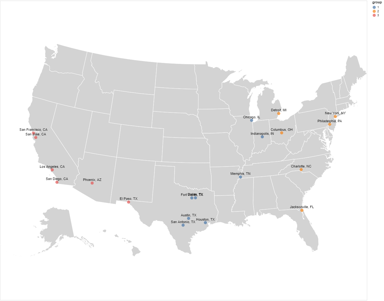
plot the cities and their groups to verify visually that they are grouped by geographic proximity.
cities.group = zeros(n)

for i in 1:n, j in 1:k
    if round(value.(x)[i,j]) == 1.0
        cities.group[i] = j
    end
end

for group in groupby(cities, :group)
    @show group
    println("")
    @show sum(group.population)
    println("")
end
group = 6×5 SubDataFrame
│ Row │ city             │ population │ lat     │ lon      │ group   │
│     │ String           │ Int64      │ Float64 │ Float64  │ Float64 │
├─────┼──────────────────┼────────────┼─────────┼──────────┼─────────┤
│ 1   │ New York, NY     │ 8405837    │ 40.7127 │ -74.0059 │ 2.0     │
│ 2   │ Philadelphia, PA │ 1553165    │ 39.9525 │ -75.1652 │ 2.0     │
│ 3   │ Jacksonville, FL │ 842583     │ 30.3321 │ -81.6556 │ 2.0     │
│ 4   │ Columbus, OH     │ 822553     │ 39.9611 │ -82.9987 │ 2.0     │
│ 5   │ Charlotte, NC    │ 792862     │ 35.227  │ -80.8431 │ 2.0     │
│ 6   │ Detroit, MI      │ 688701     │ 42.3314 │ -83.0457 │ 2.0     │

sum(group.population) = 13105701

group = 6×5 SubDataFrame
│ Row │ city              │ population │ lat     │ lon      │ group   │
│     │ String            │ Int64      │ Float64 │ Float64  │ Float64 │
├─────┼───────────────────┼────────────┼─────────┼──────────┼─────────┤
│ 1   │ Los Angeles, CA   │ 3884307    │ 34.0522 │ -118.244 │ 3.0     │
│ 2   │ Phoenix, AZ       │ 1513367    │ 33.4483 │ -112.074 │ 3.0     │
│ 3   │ San Diego, CA     │ 1355896    │ 32.7157 │ -117.161 │ 3.0     │
│ 4   │ San Jose, CA      │ 998537     │ 37.3382 │ -121.886 │ 3.0     │
│ 5   │ San Francisco, CA │ 837442     │ 37.7749 │ -122.419 │ 3.0     │
│ 6   │ El Paso, TX       │ 674433     │ 31.7775 │ -106.442 │ 3.0     │

sum(group.population) = 9263982

group = 8×5 SubDataFrame
│ Row │ city             │ population │ lat     │ lon      │ group   │
│     │ String           │ Int64      │ Float64 │ Float64  │ Float64 │
├─────┼──────────────────┼────────────┼─────────┼──────────┼─────────┤
│ 1   │ Chicago, IL      │ 2718782    │ 41.8781 │ -87.6297 │ 1.0     │
│ 2   │ Houston, TX      │ 2195914    │ 29.7604 │ -95.3698 │ 1.0     │
│ 3   │ San Antonio, TX  │ 1409019    │ 29.4241 │ -98.4936 │ 1.0     │
│ 4   │ Dallas, TX       │ 1257676    │ 32.7766 │ -96.7969 │ 1.0     │
│ 5   │ Austin, TX       │ 885400     │ 30.2671 │ -97.743  │ 1.0     │
│ 6   │ Indianapolis, IN │ 843393     │ 39.7684 │ -86.158  │ 1.0     │
│ 7   │ Fort Worth, TX   │ 792727     │ 32.7554 │ -97.3307 │ 1.0     │
│ 8   │ Memphis, TN      │ 653450     │ 35.1495 │ -90.0489 │ 1.0     │

sum(group.population) = 10756361
The populations of each group are fairly even and we can see from the plot below that the groupings look good in terms of geographic proximity: