Preliminaries
This demo presented was to the Electron Ion Collider group on April 8, 2020, before the final 1.0 version was released. Some interfaces may have changed. If you are running this notebook on Binder (i.e. you clicked on the "Launch Binder" button), then you have all the dependencies and the data file it needs to run.
Otherwise, make sure you have version 0.2.10 (GitHub, pip) by installing
pip install 'awkward1==0.2.10'
as well as the other libraries this notebook uses,
pip install 'uproot<4.0' 'particle' 'boost-histogram' 'matplotlib' 'mplhep' 'numba<0.49' 'pandas' 'numexpr' 'autograd'
and download the data file:
wget https://github.com/jpivarski/2020-04-08-eic-jlab/raw/master/open_charm_18x275_10k.root
Table of contents
- Uproot: getting data
- Awkward Array: manipulating data
- Using Uproot data in Awkward 1.0
- Iteration in Python vs array-at-a-time operations
- Zipping arrays into records and projecting them back out
- Filtering (cutting) events and particles with advanced selections
- Flattening for plots and regularizing to NumPy for machine learning
- Broadcasting flat arrays and jagged arrays
- Combinatorics: cartesian and combinations
- Reducing from combinations
- Imperative, but still fast, programming in Numba
- Grafting jagged data onto Pandas
- NumExpr, Autograd, and other third-party libraries
Uproot is a pure Python reimplementation of a significant part of ROOT I/O.
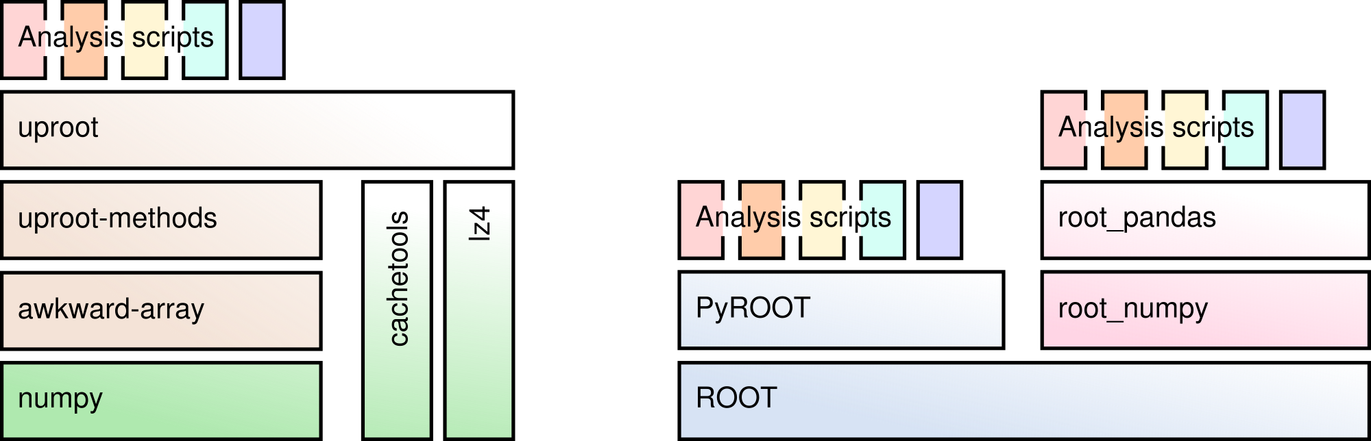
You can read TTrees containing basic data types, STL vectors, strings, and some more complex data, especially if it was written with a high "splitLevel".
You can also read histograms and other objects into generic containers, but the C++ methods that give those objects functionality are not available.
Exploring a TFile
Uproot was designed to be Pythonic, so the way we interact with ROOT files is different than it is in ROOT.
import uproot
file = uproot.open("open_charm_18x275_10k.root")
A ROOT file may be thought of as a dict of key-value pairs, like a Python dict.
file.keys()
file.values()
What's the b before the name? All strings retrieved from ROOT are unencoded, which Python 3 treats differently from Python 2. In the near future, Uproot will automatically interpret all strings from ROOT as UTF-8 and this cosmetic issue will be gone.
What's the ;1 at the end of the name? It's the cycle number, something ROOT uses to track multiple versions of an object. You can usually ignore it.
Nested directories are a dict of dicts.
file["events"].keys()
file["events"]["tree"]
But there are shortcuts:
- use a
/to navigate through the levels in a single string; - use
allkeysto recursively show all keys in all directories.
file.allkeys()
file["events/tree"]
Exploring a TTree
A TTree can also be thought of as a dict of dicts, this time to navigate through TBranches.
tree = file["events/tree"]
tree.keys()
Often, the first thing I do when I look at a TTree is show to see how each branch is going to be interpreted.
print("branch name              streamer (for complex data)  interpretation in Python")
print("==============================================================================")

tree.show()
Most of the information you'd expect to find in a TTree is there. See uproot.readthedocs.io for a complete list.
tree.numentries
tree["evt_id"].compressedbytes(), tree["evt_id"].uncompressedbytes(), tree["evt_id"].compressionratio()
tree["evt_id"].numbaskets
[tree["evt_id"].basket_entrystart(i) for i in range(3)]
Turning ROOT branches into NumPy arrays
There are several methods for this; they differ only in convenience.
# TBranch → array
tree["evt_id"].array()
# TTree + branch name → array
tree.array("evt_id")
# TTree + branch names → arrays
tree.arrays(["evt_id", "evt_prt_count"])
# TTree + branch name pattern(s) → arrays
tree.arrays("evt_*")
# TTree + branch name regex(s) → arrays
tree.arrays("/evt_[A-Z_0-9]*/i")
Convenience #1: turn the bytestrings into real strings (will soon be unnecessary).
tree.arrays("evt_*", namedecode="utf-8")
Convenience #2: output a tuple instead of a dict.
tree.arrays(["evt_id", "evt_prt_count"], outputtype=tuple)
... to use it in assignment:
evt_id, evt_prt_count = tree.arrays(["evt_id", "evt_prt_count"], outputtype=tuple)
evt_id
Memory management; caching and iteration
The array methods read an entire branch into memory. Sometimes, you might not have enough memory to do that.
The simplest solution is to set entrystart (inclusive) and entrystop (exclusive) to read a small batch at a time.
tree.array("evt_id", entrystart=500, entrystop=600)
Uproot is not agressive about caching: if you call arrays many times (for many small batches), it will read from the file every time.
You can avoid frequent re-reading by assigning arrays to variables, but then you'd have to manage all those variables.
Instead, use explicit caching:
# Make a cache with an acceptable limit.
gigabyte_cache = uproot.ArrayCache("1 GB")

# Read the array from disk:
tree.array("evt_id", cache=gigabyte_cache)

# Get the array from the cache:
tree.array("evt_id", cache=gigabyte_cache)
The advantage is that the same code can be used for first time and subsequent times. You can put this in a loop.
Naturally, fetching from the cache is much faster than reading from disk (though our file isn't very big!).
%%timeit

tree.arrays("*")
%%timeit

tree.arrays("*", cache=gigabyte_cache)
The value of an explicit cache is that you get to control it.
len(gigabyte_cache)
gigabyte_cache.clear()
len(gigabyte_cache)
Setting entrystart and entrystop can get annoying; we probably want to do it in a loop.
There's a method, iterate, for that.
for arrays in tree.iterate("evt_*", entrysteps=1000):
    print({name: len(array) for name, array in arrays.items()})
Keep in mind that this is a loop over batches, not events.
What goes in the loop is code that applies to arrays.
You can also set the entrysteps to be a size in memory.
for arrays in tree.iterate("evt_*", entrysteps="100 kB"):
    print({name: len(array) for name, array in arrays.items()})
The same size in memory covers more events if you read fewer branches.
for arrays in tree.iterate("evt_id", entrysteps="100 kB"):
    print({name: len(array) for name, array in arrays.items()})
This TTree.iterate method is similar in form to the uproot.iterate function, which iterates in batches over a collection of files.
for arrays in uproot.iterate(["open_charm_18x275_10k.root",
                              "open_charm_18x275_10k.root",
                              "open_charm_18x275_10k.root"], "events/tree", "evt_*", entrysteps="100 kB"):
    print({name: len(array) for name, array in arrays.items()})
Jagged arrays (segue)
Most of the branches in this file have an "asjagged" interpretation, instead of "asdtype" (NumPy).
tree["evt_id"].interpretation
tree["pdg"].interpretation
This means that they have multiple values per entry.
tree["pdg"].array()
Jagged arrays (lists of variable-length sublists) are very common in particle physics, and surprisingly uncommon in other fields.
We need them because we almost always have a variable number of particles per event.
from particle import Particle     # https://github.com/scikit-hep/particle

counter = 0
for event in tree["pdg"].array():
    print(len(event), "particles:", " ".join(Particle.from_pdgid(x).name for x in event))
    counter += 1
    if counter == 30:
        break
Although you can iterate over jagged arrays with for loops, the idiomatic and faster way to do it is with array-at-a-time functions.
import numpy as np

vtx_x, vtx_y, vtx_z = tree.arrays(["vtx_[xyz]"], outputtype=tuple)

vtx_dist = np.sqrt(vtx_x**2 + vtx_y**2 + vtx_z**2)

vtx_dist
import matplotlib.pyplot as plt
import mplhep as hep             # https://github.com/scikit-hep/mplhep
import boost_histogram as bh     # https://github.com/scikit-hep/boost-histogram

vtx_hist = bh.Histogram(bh.axis.Regular(100, 0, 0.1))

vtx_hist.fill(vtx_dist.flatten())

hep.histplot(vtx_hist)
vtx_dist > 0.01
pdg = tree["pdg"].array()
pdg[vtx_dist > 0.01]
counter = 0
for event in pdg[vtx_dist > 0.10]:
    print(len(event), "particles:", " ".join(Particle.from_pdgid(x).name for x in event))
    counter += 1
    if counter == 30:
        break
Particle.from_string("p~")
Particle.from_string("p~").pdgid
is_antiproton = (pdg == Particle.from_string("p~").pdgid)
is_antiproton
hep.histplot(bh.Histogram(bh.axis.Regular(100, 0, 0.1)).fill(
    vtx_dist[is_antiproton].flatten()
))
But that's a topic for the next section.
Awkward Array is a library for manipulating arbitrary data structures in a NumPy-like way.
The idea is that you have a large number of identically typed, nested objects in variable-length lists.

Using Uproot data in Awkward 1.0
Awkward Array is in transition from
- version 0.x, which is in use at the LHC but has revealed some design flaws, to
- version 1.x, which is well-architected and has completed development, but is not in widespread use yet.
Awkward 1.0 hasn't been incorporated into Uproot yet, which is how it will get in front of most users.
Since development is complete and the interface is (intentionally) different, I thought it better to show you the new version.
import awkward1 as ak
Old-style arrays can be converted into the new framework with ak.from_awkward0. This won't be a necessary step for long.
?ak.from_awkward0
?ak.to_awkward0
ak.from_awkward0(tree.array("pdg"))
arrays = {name: ak.from_awkward0(array) for name, array in tree.arrays(namedecode="utf-8").items()}
arrays
?ak.Array
Iteration in Python vs array-at-a-time operations
As before, you can iterate over them in Python, but only do that for small-scale exploration.
%%timeit -n1 -r1

vtx_dist = []
for xs, xy, xz in zip(arrays["vtx_x"], arrays["vtx_y"], arrays["vtx_z"]):
    out = []
    for x, y, z in zip(xs, xy, xz):
        out.append(np.sqrt(x**2 + y**2 + z**2))
    vtx_dist.append(out)
%%timeit -n100 -r1

vtx_dist = np.sqrt(arrays["vtx_x"]**2 + arrays["vtx_y"]**2 + arrays["vtx_z"]**2)
?ak.zip
events = ak.zip({"id": arrays["evt_id"],
                 "true": ak.zip({"q2": arrays["evt_true_q2"],
                                 "x": arrays["evt_true_x"],
                                 "y": arrays["evt_true_y"],
                                 "w2": arrays["evt_true_w2"],
                                 "nu": arrays["evt_true_nu"]}),
                 "has_dis_info": arrays["evt_has_dis_info"],
                 "prt_count": arrays["evt_prt_count"],
                 "prt": ak.zip({"id": arrays["id"],
                                "pdg": arrays["pdg"],
                                "trk_id": arrays["trk_id"],
                                "charge": arrays["charge"],
                                "dir": ak.zip({"x": arrays["dir_x"],
                                               "y": arrays["dir_y"],
                                               "z": arrays["dir_z"]}, with_name="point3"),
                                "p": arrays["p"],
                                "px": arrays["px"],
                                "py": arrays["py"],
                                "pz": arrays["pz"],
                                "m": arrays["m"],
                                "time": arrays["time"],
                                "is_beam": arrays["is_beam"],
                                "is_stable": arrays["is_stable"],
                                "gen_code": arrays["gen_code"],
                                "mother": ak.zip({"id": arrays["mother_id"],
                                                  "second_id": arrays["mother_second_id"]}),
                                "pol": ak.zip({"has_info": arrays["has_pol_info"],
                                               "x": arrays["pol_x"],
                                               "y": arrays["pol_y"],
                                               "z": arrays["pol_z"]}, with_name="point3"),
                                "vtx": ak.zip({"has_info": arrays["has_vtx_info"],
                                               "id": arrays["vtx_id"],
                                               "x": arrays["vtx_x"],
                                               "y": arrays["vtx_y"],
                                               "z": arrays["vtx_z"],
                                               "t": arrays["vtx_t"]}, with_name="point3"),
                                "smear": ak.zip({"has_info": arrays["has_smear_info"],
                                                 "has_e": arrays["smear_has_e"],
                                                 "has_p": arrays["smear_has_p"],
                                                 "has_pid": arrays["smear_has_pid"],
                                                 "has_vtx": arrays["smear_has_vtx"],
                                                 "has_any_eppid": arrays["smear_has_any_eppid"],
                                                 "orig": ak.zip({"tot_e": arrays["smear_orig_tot_e"],
                                                                 "p": arrays["smear_orig_p"],
                                                                 "px": arrays["smear_orig_px"],
                                                                 "py": arrays["smear_orig_py"],
                                                                 "pz": arrays["smear_orig_pz"],
                                                                 "vtx": ak.zip({"x": arrays["smear_orig_vtx_x"],
                                                                                "y": arrays["smear_orig_vtx_y"],
                                                                                "z": arrays["smear_orig_vtx_z"]},
                                                                               with_name="point3")})})}, with_name="particle")},
                depthlimit=1)
?ak.type
ak.type(events)
The type written with better formatting:
10000 * {"id": uint64,
         "true": {"q2": float64,
                  "x": float64,
                  "y": float64,
                  "w2": float64,
                  "nu": float64},
         "has_dis_info": int8,
         "prt_count": uint64,

         "prt": var * particle["id": uint64,
                               "pdg": int64,
                               "trk_id": float64,
                               "charge": float64,
                               "dir": point3["x": float64, "y": float64, "z": float64],
                               "p": float64,
                               "px": float64,
                               "py": float64,
                               "pz": float64,
                               "m": float64,
                               "time": float64,
                               "is_beam": bool,
                               "is_stable": bool,
                               "gen_code": bool,
                               "mother": {"id": uint64, "second_id": uint64},
                               "pol": point3["has_info": float64,
                                             "x": float64,
                                             "y": float64,
                                             "z": float64],
                               "vtx": point3["has_info": bool,
                                             "id": uint64,
                                             "x": float64,
                                             "y": float64,
                                             "z": float64,
                                             "t": float64],
                               "smear": {"has_info": bool,
                                         "has_e": bool,
                                         "has_p": bool,
                                         "has_pid": bool,
                                         "has_vtx": bool,
                                         "has_any_eppid": bool,
                                         "orig": {"tot_e":
                                                  float64,
                                                  "p": float64,
                                                  "px": float64,
                                                  "py": float64,
                                                  "pz": float64,
                                                  "vtx": point3["x": float64,
                                                                "y": float64,
                                                                "z": float64]}}]}
It means that these are now nested objects.
?ak.to_list
ak.to_list(events[0].prt[0])
ak.to_list(events[-1].prt[:10].smear.orig.vtx)
Alternatively,
ak.to_list(events[-1, "prt", :10, "smear", "orig", "vtx"])

"Zipping" arrays together into structures costs nothing (time does not scale with size of data), nor does "projecting" arrays out of structures.
events.prt.px
events.prt.py
events.prt.pz
This is called "projection" because the request for "pz" is slicing through arrays and jagged arrays.
The following are equivalent:
events[999, "prt", 12, "pz"]
events["prt", 999, 12, "pz"]
events[999, "prt", "pz", 12]
events["prt", 999, "pz", 12]
This "object oriented view" is a conceptual aid, not a constraint on computation. It's very fluid.
Moreover, we can add behaviors to named records, like methods in object oriented programming. (See ak.behavior in the documentation.)
(This is the sort of thing that a framework developer might do for the data analysts.)
def point3_absolute(data):
    return np.sqrt(data.x**2 + data.y**2 + data.z**2)

def point3_distance(left, right):
    return np.sqrt((left.x - right.x)**2 + (left.y - right.y)**2 + (left.z - right.z)**2)

ak.behavior[np.absolute, "point3"] = point3_absolute
ak.behavior[np.subtract, "point3", "point3"] = point3_distance
# Absolute value of all smear origin vertexes
abs(events.prt.smear.orig.vtx)
# Absolute value of the last smear origin vertex
abs(events[-1].prt[-1].smear.orig.vtx)
# Distance between each particle vertex and itself
events.prt.vtx - events.prt.vtx
# Distances between the first and last particle vertexes in the first 100 events
events.prt.vtx[:100, 0] - events.prt.vtx[:100, -1]
More methods can be added by declaring subclasses of arrays and records.
class ParticleRecord(ak.Record):
    @property
    def pt(self):
        return np.sqrt(self.px**2 + self.py**2)

class ParticleArray(ak.Array):
    __name__ = "Array"   # prevent it from writing <ParticleArray [...] type='...'>
                         # instead of              <Array [...] type='...'>
    @property
    def pt(self):
        return np.sqrt(self.px**2 + self.py**2)

ak.behavior["particle"] = ParticleRecord
ak.behavior["*", "particle"] = ParticleArray
type(events[0].prt[0])
events[0].prt[0]
events[0].prt[0].pt
type(events.prt)
events.prt
events.prt.pt
Filtering (cutting) events and particles with advanced selections
NumPy has a versatile selection mechanism:
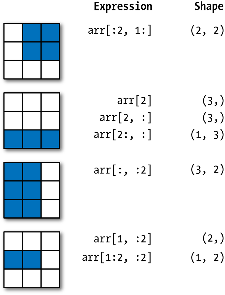
The same expressions apply to Awkward Arrays, and more.
# First particle momentum in the first 5 events
events.prt.p[:5, 0]
# First two particles in all events
events.prt.pdg[:, :2]
# First direction of the last event
events.prt.dir[-1, 0]
NumPy also lets you filter (cut) using an array of booleans.
events.prt_count > 100
np.count_nonzero(events.prt_count > 100)
events[events.prt_count > 100]
One dimension can be selected with an array while another is selected with a slice.
# Select events with at least two particles, then select the first two particles
events.prt[events.prt_count >= 2, :2]
This can be a good way to avoid errors from trying to select what isn't there.
try:
    events.prt[:, 0]
except Exception as err:
    print(type(err).__name__, str(err))
events.prt[events.prt_count > 0, 0]
See also awkward-array.readthedocs.io for a list of operations like ak.num:
?ak.num
ak.num(events.prt), events.prt_count
You can even use an array of integers to select a set of indexes at once.
# First and last particle in each event that has at least two
events.prt.pdg[ak.num(events.prt) >= 2][:, [0, -1]]
But beyond NumPy, we can also use arrays of nested lists as boolean or integer selectors.
# Array of lists of True and False
abs(events.prt.vtx) > 0.10
# Particles that have vtx > 0.10 for all events (notice that there's still 10000)
events.prt[abs(events.prt.vtx) > 0.10]
See awkward-array.readthedocs.io for more, but there are functions like ak.max, which picks the maximum in a groups.
- With
axis=0, the group is the set of all events. - With
axis=1, the groups are particles in each event.
?ak.max
ak.max(abs(events.prt.vtx), axis=1)
# Selects *events* that have a maximum *particle vertex* greater than 100
events[ak.max(abs(events.prt.vtx), axis=1) > 100]
The difference between "select particles" and "select events" is the number of jagged dimensions in the array; "reducers" like ak.max reduce the dimensionality by one.
There are other reducers like ak.any, ak.all, ak.sum...
?ak.sum
# Is this particle an antineutron?
events.prt.pdg == Particle.from_string("n~").pdgid
# Are any particles in the event antineutrons?
ak.any(events.prt.pdg == Particle.from_string("n~").pdgid, axis=1)
# Select events that contain an antineutron
events[ak.any(events.prt.pdg == Particle.from_string("n~").pdgid, axis=1)]
We can use these techniques to make subcollections for specific particle types and attach them to the same events array for easy access.
events.prt[abs(events.prt.pdg) == abs(Particle.from_string("p").pdgid)]
# Assignments have to be through __setitem__ (brackets), not __setattr__ (as an attribute).
# Is that a problem? (Assigning as an attribute would have to be implemented with care, if at all.)

events["pions"] = events.prt[abs(events.prt.pdg) == abs(Particle.from_string("pi+").pdgid)]
events["kaons"] = events.prt[abs(events.prt.pdg) == abs(Particle.from_string("K+").pdgid)]
events["protons"] = events.prt[abs(events.prt.pdg) == abs(Particle.from_string("p").pdgid)]
events.pions
events.kaons
events.protons
ak.num(events.prt), ak.num(events.pions), ak.num(events.kaons), ak.num(events.protons)
Flattening for plots and regularizing to NumPy for machine learning
All of this structure is great, but eventually, we need to plot the data or ship it to some statistical process, such as machine learning.
Most of these tools know about NumPy arrays and rectilinear data, but not Awkward Arrays.
As a design choice, Awkward Array does not implicitly flatten; you need to do this yourself, and you might make different choices of how to apply this lossy transformation in different circumstances.
The basic tool for removing structure is ak.flatten.
?ak.flatten
# Turn particles-grouped-by-event into one big array of particles
ak.flatten(events.prt, axis=1)
# Eliminate structure at all levels; produce one numerical array
ak.flatten(events.prt, axis=None)
For plotting, you probably want to pick one field and flatten it. Flattening with axis=1 (the default) works for one level of structure and is safer than axis=None.
The flattening is explicit as a reminder that a histogram whose entries are particles is different from a histogram whose entries are events.
# Directly through Matplotlib
plt.hist(ak.flatten(events.kaons.p), bins=100, range=(0, 10))
# Through mplhep and boost-histgram, which are more HEP-friendly

hep.histplot(bh.Histogram(bh.axis.Regular(100, 0, 10)).fill(

    ak.flatten(events.kaons.p)

))
If the particles are sorted (ak.sort/ak.argsort is in development), you might want to pick the first kaon from every event that has them (i.e. use the event structure).
This is an analysis choice: you have to decide you want this.
The ak.num(events.kaons) > 0 selection is explicit as a reminder that empty events are not counted in the histogram.
hep.histplot(bh.Histogram(bh.axis.Regular(100, 0, 10)).fill(

    events.kaons.p[ak.num(events.kaons) > 0, 0]

))
Or perhaps the maximum pion momentum in each event. This one must be flattened (with axis=0) to remove None values.
This flattening is explicit as a reminder that empty events are not counted in the histogram.
ak.max(events.kaons.p, axis=1)
ak.flatten(ak.max(events.kaons.p, axis=1), axis=0)
hep.histplot(bh.Histogram(bh.axis.Regular(100, 0, 10)).fill(

    ak.flatten(ak.max(events.kaons.p, axis=1), axis=0)

))
Or perhaps the momentum of the kaon with the farthest vertex. ak.argmax creates an array of integers selecting from each event.
?ak.argmax
ak.argmax(abs(events.kaons.vtx), axis=1)
?ak.singletons
# Get a length-1 list containing the index of the biggest vertex when there is one
# And a length-0 list when there isn't one
ak.singletons(ak.argmax(abs(events.kaons.vtx), axis=1))
# A nested integer array like this is what we need to select kaons with the biggest vertex
events.kaons[ak.singletons(ak.argmax(abs(events.kaons.vtx), axis=1))]
events.kaons[ak.singletons(ak.argmax(abs(events.kaons.vtx), axis=1))].p
# Flatten the distinction between length-1 lists and length-0 lists
ak.flatten(events.kaons[ak.singletons(ak.argmax(abs(events.kaons.vtx), axis=1))].p)
# Putting it all together...
hep.histplot(bh.Histogram(bh.axis.Regular(100, 0, 10)).fill(

    ak.flatten(events.kaons[ak.singletons(ak.argmax(abs(events.kaons.vtx), axis=1))].p)

))
If you're sending the data to a library that expects rectilinear structure, you might need to pad and clip the variable length lists.
ak.pad_none puts None values at the end of each list to reach a minimum length.
?ak.pad_none
# pad them                     look at the first 30
ak.pad_none(events.kaons.id, 3)[:30].tolist()
The lengths are still irregular, so you can also clip=True them.
# pad them                                look at the first 30
ak.pad_none(events.kaons.id, 3, clip=True)[:30].tolist()
The library we're sending this to might not be able to deal with missing values, so choose a replacement to fill them with.
?ak.fill_none
# fill with -1 <- pad them                                  look at the first 30
ak.fill_none(ak.pad_none(events.kaons.id, 3, clip=True), -1)[:30].tolist()
These are still Awkward-brand arrays; the downstream library might complain if they're not NumPy-brand, so use ak.to_numpy or simply cast it with NumPy's np.asarray.
?ak.to_numpy
np.asarray(ak.fill_none(ak.pad_none(events.kaons.id, 3, clip=True), -1))
If you try to convert an Awkward Array as NumPy and structure would be lost, you get an error. (You won't accidentally eliminate structure.)
try:
    np.asarray(events.kaons.id)
except Exception as err:
    print(type(err), str(err))
Broadcasting flat arrays and jagged arrays
NumPy lets you combine arrays and scalars in a mathematical expression by first "broadcasting" the scalar to an array of the same length.
print(np.array([1, 2, 3, 4, 5]) + 100)
Awkward Array does the same thing, except that each element of a flat array can be broadcasted to each nested list of a jagged array.

print(ak.Array([[1, 2, 3], [], [4, 5], [6]]) + np.array([100, 200, 300, 400]))
This is useful for emulating
all_vertices = []
for event in events:
    vertices = []
    for kaon in events.kaons:
        all_vertices.append((kaon.vtx.x - event.true.x,
                             kaon.vtx.y - event.true.y))
    all_vertices.append(vertices)
where event.true.x and y have only one value per event but kaon.vtx.x and y have one per kaon.
#       one value per kaon   one per event
ak.zip([events.kaons.vtx.x - events.true.x,
        events.kaons.vtx.y - events.true.y])
You don't have to do anything special for this: broadcasting is a common feature of all functions that apply to more than one array.
You can get it explicitly with ak.broadcast_arrays.
?ak.broadcast_arrays
ak.broadcast_arrays(events.true.x, events.kaons.vtx.x)
Combinatorics: cartesian and combinations
At all levels of a physics analysis, we need to compare objects drawn from different collections.
- Gen-reco matching: to associate a reconstructed particle with its generator-level parameters.
- Cleaning: assocating soft photons with a reconstructed electron or leptons to a jet.
- Bump-hunting: looking for mass peaks in pairs of particles.
- Dalitz analysis: looking for resonance structure in triples of particles.
To do this with array-at-a-time operations, use one function to generate all the combinations,

apply "flat" operations,

then use "reducers" to get one value per particle or per event again.

Cartesian and combinations
The two main "explode" operations are ak.cartesian and ak.combinations.
The first generates the Cartesian product (a.k.a. cross product) of two collections per nested list.

The second generates distinct combinations (i.e. "n choose k") of a collection with itself per nested list.

?ak.cartesian
?ak.combinations
ak.to_list(ak.cartesian(([[1, 2, 3], [], [4]],
                         [["a", "b"], ["c"], ["d", "e"]])))
ak.to_list(ak.combinations([["a", "b", "c", "d"], [], [1, 2]], 2))
To search for $\Lambda^0 \to \pi p$, we need to compute the mass of pairs drawn from these two collections.
pairs = ak.cartesian([events.pions, events.protons])
pairs
?ak.unzip
def mass(pairs, left_mass, right_mass):
    left, right = ak.unzip(pairs)
    left_energy = np.sqrt(left.p**2 + left_mass**2)
    right_energy = np.sqrt(right.p**2 + right_mass**2)
    return np.sqrt((left_energy + right_energy)**2 -
                   (left.px + right.px)**2 -
                   (left.py + right.py)**2 -
                   (left.pz + right.pz)**2)
mass(pairs, 0.139570, 0.938272)
hep.histplot(bh.Histogram(bh.axis.Regular(100, 1.115683 - 0.01, 1.115683 + 0.01)).fill(
    ak.flatten(mass(pairs, 0.139570, 0.938272))
))
We can improve the peak by selecting for opposite charges and large vertexes.
def opposite(pairs):
    left, right = ak.unzip(pairs)
    return pairs[left.charge != right.charge]

def distant(pairs):
    left, right = ak.unzip(pairs)
    return pairs[np.logical_and(abs(left.vtx) > 0.10, abs(right.vtx) > 0.10)]
hep.histplot(bh.Histogram(bh.axis.Regular(100, 1.115683 - 0.01, 1.115683 + 0.01)).fill(
    ak.flatten(mass(distant(opposite(pairs)), 0.139570, 0.938272))
))
Alternatively, all of these functions could have been methods on the pair objects for reuse.
(This is to make the point that any kind of object can have methods, not just particles.)
class ParticlePairArray(ak.Array):
    __name__ = "Pairs"

    def mass(self, left_mass, right_mass):
        left, right = self.slot0, self.slot1
        left_energy = np.sqrt(left.p**2 + left_mass**2)
        right_energy = np.sqrt(right.p**2 + right_mass**2)
        return np.sqrt((left_energy + right_energy)**2 -
                       (left.px + right.px)**2 -
                       (left.py + right.py)**2 -
                       (left.pz + right.pz)**2)

    def opposite(self):
        return self[self.slot0.charge != self.slot1.charge]

    def distant(self, cut):
        return self[np.logical_and(abs(self.slot0.vtx) > cut, abs(self.slot1.vtx) > cut)]

ak.behavior["*", "pair"] = ParticlePairArray
pairs = ak.cartesian([events.pions, events.protons], with_name="pair")
pairs
hep.histplot(bh.Histogram(bh.axis.Regular(100, 1.115683 - 0.01, 1.115683 + 0.01)).fill(
    ak.flatten(pairs.opposite().distant(0.10).mass(0.139570, 0.938272))
))
Self-study question: why does the call to mass have to be last?
An example for ak.combinations: $K_S \to \pi\pi$.
pairs = ak.combinations(events.pions, 2, with_name="pair")
pairs
hep.histplot(bh.Histogram(bh.axis.Regular(100, 0.497611 - 0.015, 0.497611 + 0.015)).fill(
    ak.flatten(pairs.opposite().distant(0.10).mass(0.139570, 0.139570))
))
Bonus problem: $D^0 \to K^- \pi^+ \pi^0$
pizero_candidates = ak.combinations(events.prt[events.prt.pdg == Particle.from_string("gamma").pdgid], 2, with_name="pair")
pizero = pizero_candidates[pizero_candidates.mass(0, 0) - 0.13498 < 0.000001]
pizero["px"] = pizero.slot0.px + pizero.slot1.px
pizero["py"] = pizero.slot0.py + pizero.slot1.py
pizero["pz"] = pizero.slot0.pz + pizero.slot1.pz
pizero["p"] = np.sqrt(pizero.px**2 + pizero.py**2 + pizero.pz**2)
pizero
kminus = events.prt[events.prt.pdg == Particle.from_string("K-").pdgid]
piplus = events.prt[events.prt.pdg == Particle.from_string("pi+").pdgid]

triples = ak.cartesian({"kminus": kminus[abs(kminus.vtx) > 0.03],
                        "piplus": piplus[abs(piplus.vtx) > 0.03],
                        "pizero": pizero[np.logical_and(abs(pizero.slot0.vtx) > 0.03, abs(pizero.slot1.vtx) > 0.03)]})
triples
ak.num(triples)
def mass2(left, left_mass, right, right_mass):
    left_energy = np.sqrt(left.p**2 + left_mass**2)
    right_energy = np.sqrt(right.p**2 + right_mass**2)
    return ((left_energy + right_energy)**2 -
            (left.px + right.px)**2 -
            (left.py + right.py)**2 -
            (left.pz + right.pz)**2)
mKpi = mass2(triples.kminus, 0.493677, triples.piplus, 0.139570)
mpipi = mass2(triples.piplus, 0.139570, triples.pizero, 0.1349766)
This Dalitz plot doesn't look right (doesn't cut off at kinematic limits), but I'm going to leave it as an exercise for the reader.
dalitz = bh.Histogram(bh.axis.Regular(50, 0, 3), bh.axis.Regular(50, 0, 2))
dalitz.fill(ak.flatten(mKpi), ak.flatten(mpipi))

X, Y = dalitz.axes.edges

fig, ax = plt.subplots()
mesh = ax.pcolormesh(X.T, Y.T, dalitz.view().T)
fig.colorbar(mesh)
Reducing from combinations
The mass-peak examples above don't need to "reduce" combinations, but many applications do.
Suppose that we want to find the "nearest photon to each electron" (e.g. bremsstrahlung).
electrons = events.prt[abs(events.prt.pdg) == abs(Particle.from_string("e-").pdgid)]
photons   = events.prt[events.prt.pdg == Particle.from_string("gamma").pdgid]
The problem with the raw output of ak.cartesian is that all the combinations are mixed together in the same lists.
ak.to_list(ak.cartesian([electrons[["pdg", "id"]], photons[["pdg", "id"]]])[8])
We can fix this by asking for nested=True, which adds another level of nesting to the output.
ak.to_list(ak.cartesian([electrons[["pdg", "id"]], photons[["pdg", "id"]]], nested=True)[8])
All electron-photon pairs associated with a given electron are grouped in a list-within-each-list.
Now we can apply reducers to this inner dimension to sum over some quantity, pick the best one, etc.
def cos_angle(pairs):
    left, right = ak.unzip(pairs)
    return left.dir.x*right.dir.x + left.dir.y*right.dir.y + left.dir.z*right.dir.z
electron_photons = ak.cartesian([electrons, photons], nested=True)
cos_angle(electron_photons)
hep.histplot(bh.Histogram(bh.axis.Regular(100, -1, 1)).fill(
    ak.flatten(cos_angle(electron_photons), axis=None)    # a good reason to use flatten axis=None
))
We pick the "maximum according to a function" using the same ak.singletons(ak.argmax(f(x)) trick as above.
best_electron_photons = electron_photons[ak.singletons(ak.argmax(cos_angle(electron_photons), axis=2))]

hep.histplot(bh.Histogram(bh.axis.Regular(100, -1, 1)).fill(
    ak.flatten(cos_angle(best_electron_photons), axis=None)
))
By construction, best_electron_photons has zero or one elements in each inner nested list.
ak.num(electron_photons, axis=2), ak.num(best_electron_photons, axis=2)
Since we no longer care about that inner structure, we could flatten it at axis=2 (leaving axis=1 untouched).
best_electron_photons
ak.flatten(best_electron_photons, axis=2)
But it would be better to invert the ak.singletons by calling ak.firsts.
?ak.singletons
?ak.firsts
ak.firsts(best_electron_photons, axis=2)
Because then we can get back one value for each electron (with None if ak.argmax resulted in None because there were no pairs).
ak.num(electrons), ak.num(ak.firsts(best_electron_photons, axis=2))
ak.all(ak.num(electrons) == ak.num(ak.firsts(best_electron_photons, axis=2)))
And that means that we can make this "closest photon" an attribute of the electrons. We have now performed electron-photon matching.
electrons["photon"] = ak.firsts(best_electron_photons, axis=2)
ak.to_list(electrons[8])
Current set of reducers:
- ak.count: counts the number in each group (subtly different from ak.num because
ak.countis a reducer) - ak.count_nonzero: counts the number of non-zero elements in each group
- ak.sum: adds up values in the group, the quintessential reducer
- ak.prod: multiplies values in the group (e.g. for charges or probabilities)
- ak.any: boolean reducer for logical
or("do any in this group satisfy a constraint?") - ak.all: boolean reducer for logical
and("do all in this group satisfy a constraint?") - ak.min: minimum value in each group (
Nonefor empty groups) - ak.max: maximum value in each group (
Nonefor empty groups) - ak.argmin: index of minimum value in each group (
Nonefor empty groups) - ak.argmax: index of maximum value in each group (
Nonefor empty groups)
And other functions that have the same interface as a reducer (reduces a dimension):
- ak.moment: computes the $n^{th}$ moment in each group
- ak.mean: computes the mean in each group
- ak.var: computes the variance in each group
- ak.std: computes the standard deviation in each group
- ak.covar: computes the covariance in each group
- ak.corr: computes the correlation in each group
- ak.linear_fit: computes the linear fit in each group
- ak.softmax: computes the softmax function in each group
Imperative, but still fast, programming in Numba
Array-at-a-time operations let us manipulate dynamically typed data with compiled code (and in some cases, benefit from hardware vectorization). However, they're complicated. Finding the closest photon to each electron is more complicated than it seems it ought to be.
Some of these things are simpler in imperative (step-by-step scalar-at-a-time) code. Imperative Python code is slow because it has to check the data type of every object it enounters (among other things); compiled code is faster because these checks are performed once during a compilation step for any number of identically typed values.
We can get the best of both worlds by Just-In-Time (JIT) compiling the code. Numba is a NumPy-centric JIT compiler for Python.
import numba as nb

@nb.jit
def monte_carlo_pi(nsamples):
    acc = 0
    for i in range(nsamples):
        x = np.random.random()
        y = np.random.random()
        if (x**2 + y**2) < 1.0:
            acc += 1
    return 4.0 * acc / nsamples
%%timeit

# Run the pure Python function (without nb.jit)
monte_carlo_pi.py_func(1000000)
%%timeit

# Run the compiled function
monte_carlo_pi(1000000)
The price for this magical speedup is that not all Python code can be accelerated; you have to be conservative with the functions and language features you use, and Numba has to recognize the data types.
Numba recognizes Awkward Arrays.
@nb.jit
def lambda_mass(events):
    num_lambdas = 0
    for event in events:
        num_lambdas += len(event.pions) * len(event.protons)

    lambda_masses = np.empty(num_lambdas, np.float64)
    i = 0
    for event in events:
        for pion in event.pions:
            for proton in event.protons:
                pion_energy = np.sqrt(pion.p**2 + 0.139570**2)
                proton_energy = np.sqrt(proton.p**2 + 0.938272**2)
                mass = np.sqrt((pion_energy + proton_energy)**2 -
                               (pion.px + proton.px)**2 -
                               (pion.py + proton.py)**2 -
                               (pion.pz + proton.pz)**2)
                lambda_masses[i] = mass
                i += 1

    return lambda_masses

lambda_mass(events)
hep.histplot(bh.Histogram(bh.axis.Regular(100, 1.115683 - 0.01, 1.115683 + 0.01)).fill(
    lambda_mass(events)
))
Some constraints:
- Awkward arrays are read-only structures (always true, even outside of Numba)
- Awkward arrays can't be created inside a Numba-compiled function
That was fine for a function that creates and returns a NumPy array, but what if we want to create something with structure?
The ak.ArrayBuilder is a general way to make data structures.
?ak.ArrayBuilder
builder = ak.ArrayBuilder()

builder.begin_list()

builder.begin_record()
builder.field("x").integer(1)
builder.field("y").real(1.1)
builder.field("z").string("one")
builder.end_record()

builder.begin_record()
builder.field("x").integer(2)
builder.field("y").real(2.2)
builder.field("z").string("two")
builder.end_record()

builder.end_list()

builder.begin_list()
builder.end_list()

builder.begin_list()

builder.begin_record()
builder.field("x").integer(3)
builder.field("y").real(3.3)
builder.field("z").string("three")
builder.end_record()

builder.end_list()

ak.to_list(builder.snapshot())
ArrayBuilders can be used in Numba, albeit with some constraints:
- ArrayBuilders can't be created inside a Numba-compiled function (pass them in)
- The
snapshotmethod (to turn it into an array) can't be used in a Numba-compiled function (use it outside)
@nb.jit(nopython=True)
def make_electron_photons(events, builder):
    for event in events:
        builder.begin_list()
        for electron in event.electrons:
            best_i = -1
            best_angle = -1.0
            for i in range(len(event.photons)):
                photon = event.photons[i]
                angle = photon.dir.x*electron.dir.x + photon.dir.y*electron.dir.y + photon.dir.z*electron.dir.z
                if angle > best_angle:
                    best_i = i
                    best_angle = angle
            if best_i == -1:
                builder.null()
            else:
                builder.append(photon)
        builder.end_list()

events["electrons"] = events.prt[abs(events.prt.pdg) == abs(Particle.from_string("e-").pdgid)]
events["photons"]   = events.prt[events.prt.pdg == Particle.from_string("gamma").pdgid]

builder = ak.ArrayBuilder()
make_electron_photons(events, builder)
builder.snapshot()
A few of them are None (called builder.null() because there were no photons to attach to the electron).
ak.count_nonzero(ak.is_none(ak.flatten(builder.snapshot())))
But the builder.snapshot() otherwise matches up with the events.electrons, so it's something we could attach to it, as before.
?ak.with_field
events["electrons"] = ak.with_field(events.electrons, builder.snapshot(), "photon")
ak.to_list(events[8].electrons)
Grafting jagged data onto Pandas
Awkward Arrays can be Pandas columns.
import pandas as pd

df = pd.DataFrame({"pions": events.pions,
                   "kaons": events.kaons,
                   "protons": events.protons})
df
df["pions"].dtype
But that's unlikely to be useful for very complex data structures because there aren't any Pandas functions for deeply nested structure.
Instead, you'll probably want to convert the nested structures into the corresponding Pandas MultiIndex.
?ak.pandas.df
ak.pandas.df(events.pions)
Now the nested lists are represented as MultiIndex rows and the nested records are represented as MultiIndex columns, which are structures that Pandas knows how to deal with.
But what about two types of particles, pions and kaons? (And let's simplify to just "px", "py", "pz", "vtx".)
simpler = ak.zip({"pions": events.pions[["px", "py", "pz", "vtx"]],
                  "kaons": events.kaons[["px", "py", "pz", "vtx"]]}, depthlimit=1)
ak.type(simpler)
ak.pandas.df(simpler)
There's only one row MultiIndex, so pion #1 in each event is the same row as kaon #1. That assocation is probably meaningless.
The issue is that a single Pandas DataFrame represents less information than an Awkward Array. In general, we would need a collection of DataFrames to losslessly encode an Awkward Array. (Pandas represents the data in database normal form; Awkward represents it in objects.)
?ak.pandas.dfs
# This array corresponds to *two* Pandas DataFrames.
pions_df, kaons_df = ak.pandas.dfs(simpler)
pions_df
kaons_df
NumExpr, Autograd, and other third-party libraries
NumExpr can calcuate pure numerical expressions faster than NumPy because it does so in one pass. (It has a low-overhead virtual machine.)
NumExpr doesn't recognize Awkward Arrays, but we have a wrapper for it.
import numexpr

# This works because px, py, pz are flat, like NumPy
px = ak.flatten(events.pions.px)
py = ak.flatten(events.pions.py)
pz = ak.flatten(events.pions.pz)
numexpr.evaluate("px**2 + py**2 + pz**2")
# This doesn't work because px, py, pz have structure
px = events.pions.px
py = events.pions.py
pz = events.pions.pz
try:
    numexpr.evaluate("px**2 + py**2 + pz**2")
except Exception as err:
    print(type(err), str(err))
# But in this wrapped version, we broadcast and maintain structure
ak.numexpr.evaluate("px**2 + py**2 + pz**2")
Similarly for Autograd, which has an elementwise_grad for differentiating expressions with respect to NumPy universal functions, but not Awkward Arrays.
@ak.autograd.elementwise_grad
def tanh(x):
    y = np.exp(-2.0 * x)
    return (1.0 - y) / (1.0 + y)

ak.to_list(tanh([{"x": 0.0, "y": []}, {"x": 0.1, "y": [1]}, {"x": 0.2, "y": [2, 2]}, {"x": 0.3, "y": [3, 3, 3]}]))
The set of third-party libraries supported this way will continue to grow. Some major plans on the horizon:
- Apache Arrow, and through it the Parquet file format.
- The Zarr array delivery system.
- CuPy and Awkward Arrays on the GPU.