LISSOM's weights and activations
This notebook plots the weights and activations of different LISSOM layers:
- Cortex: a torch.Linear layer with special initilization and connective radius, to represent an afferent, excitatory or inhibitory map
- LGN: a layer representing the Lateral Geniculate Nucleus of the brain.
- ReducedLissom: combines the activation of three cortex layers as lateral interactions of the same map, representing the V1 of the brain
- Lissom: combines the activation one ReducedLissom and two LGN's, a model of the full visual processing till the V1
REMARK: All ipynb's except OrientationMaps instantiate each layer explicitly with the neccesary arguments, to show all the params. For complex layers, they are a lot, but pylissom provides a tool for simplifying this, reading from a config file, akin to pytorch model zoo. For this and other helpful tools, please check the Orientation Maps ipynb and the documentation page.
from pylissom.nn.modules.lissom import *
from pylissom.nn.modules import register_recursive_input_output_hook
from pylissom.utils.plotting import *
from pylissom.utils.stimuli import gaussian_generator

import matplotlib.pyplot as plt
Inspecting a Cortex layer’s weights
Here, we build a cortex layer of dimension 5x5. This layer receive its input from an input layer of dimension 25x25. Each cortex neuron will have a receptive field of radius 5. The connection weights are initialized with a Gaussian function of $\sigma = 5$.
in_features = 25**2
out_features = 5**2
cortex = Cortex(in_features, out_features, radius=5, sigma=5)
Next, we plot in grayscale the layer's initial weights using the plot_layer_weights helper function.
As the dimension of V1 is 5x5, there are 25 neurons in V1. The plot shows the initial weights for each of these neurons, in a 5x5 array. Each neuron has 25x25 square plot, representing the retina. The weights are seen as clouds of white dots. As each neuron has a receptive field of radius 5, circular white plots of radius 5 are observed in the figure. However, most of the 25x25 weights of each neuron are equal to zero because they are outside the receptive field of the neuron, which explains the plot’s darkness
plt.figure(figsize=(12, 12))
plot_layer_weights(cortex, use_range=False)

To make this more clear, now we plot a pylissom.nn.linear.GaussianCloud layer that has the same initial weights as the cortex but without the receptive field limitation. As we can see, the white dots clouds are larger and brighter than the ones in the previous figure. The clouds are larger, because there is not the receptive field limitation. The clouds are brighter because there is not the normalization process that is done in the Cortex layer. Each weight in the GaussianCloud layer can have values between 0 and 1 but for a Cortex neuron, the sum of all weights must equal 1, so most weights have very small values, decaying proportionally to the size of the receptive field, hence the darkness.
gaussian_linear = GaussianCloudLinear(in_features, out_features, sigma=5)
plt.figure(figsize=(12, 12))
plot_layer_weights(gaussian_linear)

DiffOfGaussians
Next we plot the weights of the DifferenceOfGaussiansLinear layer, the basis on which the LGN layer is built. The initialization is different than the previous cortex layer. As explained in the Test_simple_modules ipynb, the weights are the difference of two gaussian weights matrix with different $\sigma$.
We plot first the weights of the DifferenceOfGaussiansLinear. The plot is in grey because the LGN weights are between -1 and 1, as oppose to cortex which are 0 and 1.
The DoGLinear is the same layer as UnnormalizedDifferenceOfGaussiansLinear (the next plot) but with the connective radius and normalization applied. The same characteristic that happened with Cortex appears, with a brighter plot than the original.
in_features = 25**2
out_features = 5**2
dofg = DifferenceOfGaussiansLinear(in_features, out_features, radius=5, on=False, sigma_surround=5, sigma_center=1)
plt.figure(figsize=(12, 12))
plot_layer_weights(dofg, use_range=True)

in_features = 24**2
out_features = 5**2
unnorm_dofg = UnnormalizedDifferenceOfGaussiansLinear(in_features, out_features, on=False, sigma_surround=5, sigma_center=1)
plt.figure(figsize=(12, 12))
plot_layer_weights(unnorm_dofg, use_range=True)

LGN
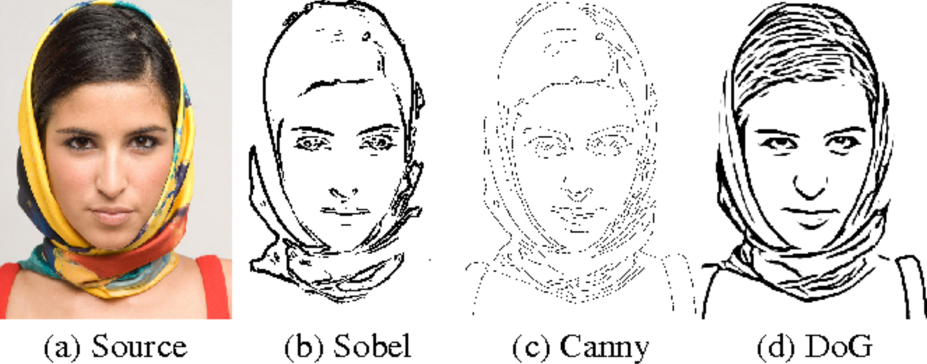
An LGN layer applies a PiecewiseSigmoid (see Tests_simple_modules ipynb) to a DifferenceOfGaussiansLinear activation. It models an edge-detection mechanism that happens in the brain.
This is an ilustrative example of some edge detection filters, with DoG in (d). The image was not done with pytorch
retinal_density = 36
lgn_density = 36
radius_afferent = (lgn_density / 4 + 0.5)
scale_afferent = radius_afferent / 6.5  # radius_afferent_reference
radius_center_gaussian = 0.5*scale_afferent*retinal_density/lgn_density
radius_surround_gaussian = 4*radius_center_gaussian
radius_afferent_lgn = 4.7*radius_surround_gaussian
in_features = retinal_density **2
out_features = lgn_density**2
off_test = LGN(in_features, out_features,
          on=False,
          radius=radius_afferent_lgn,
                    sigma_surround=5, sigma_center=2)
on_test = LGN(in_features, out_features,
          on=True,
          radius=radius_afferent_lgn,
          sigma_surround=radius_surround_gaussian, sigma_center=radius_center_gaussian)
Input to the LGN, a gaussian stimulus:
gauss_size = int(in_features**0.5)
sigma_x = 3
sigma_y = sigma_x
gauss = gaussian_generator(gauss_size, gauss_size//2, gauss_size//2, sigma_x, sigma_y, 0)
plot_matrix(gauss)
inp = torch.autograd.Variable(torch.from_numpy(gauss).view(in_features)).unsqueeze(0)

As we see here, the LGN enhances the edges of the gaussian input
out_rows = int(out_features**0.5)
out = (on_test(inp) - off_test(inp)).data*2.33/1
mat = tensor_to_numpy_matrix(out, (out_rows,out_rows))
plt.imshow(mat, cmap='gray', vmin=-0.5, vmax=0.5)
plt.show()

Inspecting a layer’s activation: ReducedLissom
For this example, we will use a pylissom.nn.lissom.ReducedLissom layer to inspect the activation of its neurons. A ReducedLissom represents the V1 of the brain. A composition approach was used for complex layers such as ReducedLissom, so the parameters, in this case, are the afferent, excitatory and inhibitory modules (which are Cortex layers) already initialized, and also the strength factors, the settling steps and the $\theta$ threshold values for the Piecewise Sigmoid activation function.
In essence this ReducedLissom layer implements the lateral interactions of the full LISSOM model, and abstracts itself from the creation of the inner cortex layers.
The V1 layer, has a 36x36 dimension. The retina layer has also 36x36 dimension. Other parameters needed to build the ReducedLissom are listed below:
retinal_density = 36
lgn_density = retinal_density
cortical_density = 36
# Receptive Fields
radius_afferent = (lgn_density / 4 + 0.5)
radius_excitatory = (cortical_density / 10)
radius_inhibitory = cortical_density / 4 - 1
radius_gaussian_afferent = radius_afferent / 1.3
radius_gaussian_excitatory = 0.78 * radius_excitatory
radius_gaussian_inhibitory = 2.08 * radius_inhibitory
# Activation
settling_steps = 9
min_theta = 0.083
max_theta = min_theta + 0.55
# Scaling
afferent_factor = 1.0
excitatory_factor = 0.9
inhibitory_factor = 0.9
in_features = lgn_density**2
out_features = cortical_density**2
excitatory_map = Cortex(in_features, out_features, radius=radius_excitatory, sigma=radius_gaussian_excitatory)
in_features = cortical_density**2
out_features = cortical_density**2
afferent_map = Cortex(in_features, out_features, radius=radius_afferent, sigma=radius_gaussian_afferent)
in_features = cortical_density**2
out_features = cortical_density**2
inhibitory_map = Cortex(in_features, out_features, radius=radius_inhibitory, sigma=radius_gaussian_inhibitory)
Here, we build ReducedLissom:
v1 = ReducedLissom(afferent_module=afferent_map, excitatory_module=excitatory_map, inhibitory_module=inhibitory_map,
                   min_theta=min_theta, max_theta=max_theta, settling_steps=settling_steps,
                  inhibitory_strength=inhibitory_factor, afferent_strength=afferent_factor,
                   excitatory_strength=excitatory_factor)
The different internal parameters of ReducedLissom are displayed:
print(repr(v1))
ReducedLissom (
  (inhibitory_module): Cortex (1296 -> 1296, sigma=16.64, radius=8.0)
  (excitatory_module): Cortex (1296 -> 1296, sigma=2.8080000000000003, radius=3.6)
  (afferent_module): Cortex (1296 -> 1296, sigma=7.3076923076923075, radius=9.5)
  (piecewise_sigmoid): PiecewiseSigmoid (min_theta=0.083, max_theta=0.633)
, 1296 -> 1296, settling_steps=9, afferent_strength=1.0, excitatory_strength=0.9, inhibitory_strength=0.9)
Hooks to the module for plotting the input and activation of each submodule
register_recursive_input_output_hook(v1)
[<torch.utils.hooks.RemovableHandle at 0x7f8b182a3898>,
 <torch.utils.hooks.RemovableHandle at 0x7f8b182a3828>,
 <torch.utils.hooks.RemovableHandle at 0x7f8b18311da0>,
 <torch.utils.hooks.RemovableHandle at 0x7f8b18311cc0>,
 <torch.utils.hooks.RemovableHandle at 0x7f8b18311cf8>]
Here we create a gaussian input stimuli using the gaussian_generator helper function, that must match the retina size:
gauss_size = int(in_features**0.5)
gauss = gaussian_generator(gauss_size, gauss_size//2, gauss_size//2, 2, 2, 0)
plot_matrix(gauss)

Now we transform the numpy array to a pytorch Variable and resize it to match the 1-dimensional shape that pytorch layers expect as input.
inp = torch.autograd.Variable(torch.from_numpy(gauss).view(in_features)).unsqueeze(0)
A plot of the ReducedLissom activation for the gaussian stimulus is displayed below. Note that the activations for all the neurons in the V1 layer are displayed, because the V1 has a 36x36 dimension.
out_rows = int(out_features**0.5)
plot_tensor(v1(inp*2.33).data, (out_rows,out_rows))

Below we plot the input and activation for the different modules that contribute to the activation of a V1 neuron:
- v1.inhibitory_module.input: input at time (t-1) for the inhibitory connections. These are the activations of the V1 neurons at time (t-1).
- v1.inhibitory_module.activation: these is the product of the input at time (t-1) and the inhibitory weights.
- v1.excitatory_module.input: input at time (t-1) for the excitatory connections. These are the activations of the V1 neurons at time (t-1). Note that this is the same figure than the top figure, because the input is the activation of the V1 neurons at time (t-1).
- v1.excitatory_module.activation: these is the product of the input at time (t-1) and the excitatory weights.
- v1.afferent_module.input: input at the retina.
- v1.afferent_module.activation: these is the product of the input at the retina and the afferent weights.
- v1.input: input at the retina.
- v1.activation: final activation of the V1 layer at time t.
plot_layer_activation(v1, 'v1')


Lissom
As explained before, LISSOM models the visual processing of the brain till the V1.
For this, it has the two previous LGN layers, called on and off, and a ReducedLissom layer, the v1. The activation is just $v1(on(retina\_input) + off(retina\_input))$, meaing: first we calculate the sum of the channels activations to the input, and then passed it trough the v1.
retinal_density = 36
lgn_density = 36
cortical_density = 36
# Receptive Fields
radius_afferent = (lgn_density / 4 + 0.5)
radius_excitatory = (cortical_density / 10)
radius_inhibitory = cortical_density / 4 - 1
radius_gaussian_afferent = radius_afferent / 1.3
radius_gaussian_excitatory = 0.78 * radius_excitatory
radius_gaussian_inhibitory = 2.08 * radius_inhibitory
# LGN
scale_afferent = radius_afferent / 6.5  # radius_afferent_reference
radius_center_gaussian = 0.5*scale_afferent*retinal_density/lgn_density
radius_surround_gaussian = 4*radius_center_gaussian
radius_afferent_lgn = 4.7*radius_surround_gaussian
# Activation
settling_steps = 9
min_theta = 0.083
max_theta = min_theta + 0.55
# Scaling
afferent_factor = 1.0
excitatory_factor = 0.9
inhibitory_factor = 0.9
lgn_factor = 2.33 / 1 #  (brightness scale of the retina, contrast of fully bright stimulus)
in_features = lgn_density**2
out_features = cortical_density**2
excitatory_map = Cortex(in_features, out_features, radius=radius_excitatory, sigma=radius_gaussian_excitatory)
in_features = cortical_density**2
out_features = cortical_density**2
afferent_map = Cortex(in_features, out_features, radius=radius_afferent, sigma=radius_gaussian_afferent)
in_features = cortical_density**2
out_features = cortical_density**2
inhibitory_map = Cortex(in_features, out_features, radius=radius_inhibitory, sigma=radius_gaussian_inhibitory)
v1 = ReducedLissom(afferent_module=afferent_map, excitatory_module=excitatory_map, inhibitory_module=inhibitory_map,
                   min_theta=min_theta, max_theta=max_theta, settling_steps=settling_steps,
                  inhibitory_strength=inhibitory_factor, afferent_strength=afferent_factor,
                   excitatory_strength=excitatory_factor)
in_features = retinal_density **2
out_features = lgn_density**2
off = LGN(in_features, out_features,
          on=False,
          radius=radius_afferent_lgn,
                    sigma_surround=radius_surround_gaussian, sigma_center=radius_center_gaussian,
         strength=lgn_factor)
on = LGN(in_features, out_features,
          on=True,
          radius=radius_afferent_lgn,
          sigma_surround=radius_surround_gaussian, sigma_center=radius_center_gaussian,
        strength=lgn_factor)
lissom = Lissom(on=on, off=off, v1=v1)
print(repr(lissom))
Lissom (
  (v1): ReducedLissom (
    (inhibitory_module): Cortex (1296 -> 1296, sigma=16.64, radius=8.0)
    (excitatory_module): Cortex (1296 -> 1296, sigma=2.8080000000000003, radius=3.6)
    (afferent_module): Cortex (1296 -> 1296, sigma=7.3076923076923075, radius=9.5)
    (piecewise_sigmoid): PiecewiseSigmoid (min_theta=0.083, max_theta=0.633)
  , 1296 -> 1296, settling_steps=9, afferent_strength=1.0, excitatory_strength=0.9, inhibitory_strength=0.9)
  (off): LGN (
    (diff_of_gaussians): DifferenceOfGaussiansLinear (1296 -> 1296, sigma_surround=2.923076923076923, sigma_center=0.7307692307692307, radius=13.738461538461538, on=False)
    (strength): *2.33
    (piecewise_sigmoid): PiecewiseSigmoid (min_theta=0.0, max_theta=1.0)
  )
  (on): LGN (
    (diff_of_gaussians): DifferenceOfGaussiansLinear (1296 -> 1296, sigma_surround=2.923076923076923, sigma_center=0.7307692307692307, radius=13.738461538461538, on=True)
    (strength): *2.33
    (piecewise_sigmoid): PiecewiseSigmoid (min_theta=0.0, max_theta=1.0)
  )
, 1296 -> 1296)
register_recursive_forward_hook(lissom, input_output_hook)
gauss_size = int(in_features**0.5)
gauss = gaussian_generator(gauss_size, gauss_size//2, gauss_size//2, 2, 2, 0)
plot_matrix(gauss)
inp = torch.autograd.Variable(torch.from_numpy(gauss).view(in_features)).unsqueeze(0)
out_rows = int(out_features**0.5)
plot_tensor(lissom(inp).data, (out_rows,out_rows))

plot_layer_activation(lissom, 'lissom')
Playground