Topological feature extraction from graphs
giotto-tda can extract topological features from undirected or directed graphs represented as adjacency matrices, via the following transformers:
- VietorisRipsPersistence and SparseRipsPersistence initialized with
metric="precomputed", for undirected graphs; - FlagserPersistence initialized with
directed=True, for directed graphs, and withdirected=Falsefor undirected ones.
In this notebook, we build some basic intuition on how these methods are able to capture structures and patterns from such graphs. We will focus on the multi-scale nature of the information contained in the final outputs ("persistence diagrams"), as well as on the differences between the undirected and directed cases. Although adjacency matrices of sparsely connected and even unweighted graphs can be passed directly to these transformers, they are interpreted as weighted adjacency matrices according to some non-standard conventions. We will highlight these conventions below.
The mathematical technologies used under the hood are various flavours of "persistent homology" (as is also the case for EuclideanCechPersistence and CubicalPersistence). If you are interested in the details, you can start from the theory glossary and references therein.
If you are looking at a static version of this notebook and would like to run its contents, head over to GitHub and download the source.
See also
- Topological feature extraction using VietorisRipsPersistence and PersistenceEntropy which treats the "special case" of point clouds (see below).
- Plotting in giotto-tda, particularly Section 1.2 (as above, treats the case of point clouds).
- Classifying 3D shapes (a more advanced example).
- Computing persistent homology of directed flag complexes by Daniel Luetgehetmann, Dejan Govc, Jason Smith, and Ran Levi.
License: AGPLv3
Import libraries
import numpy as np
from numpy.random import default_rng
rng = default_rng(42)  # Create a random number generator

from scipy.spatial.distance import pdist, squareform
from scipy.sparse import csr_matrix

from gtda.graphs import GraphGeodesicDistance
from gtda.homology import VietorisRipsPersistence, SparseRipsPersistence, FlagserPersistence

from igraph import Graph

from IPython.display import SVG, display
Undirected graphs – VietorisRipsPersistence and SparseRipsPersistence
General API
If you have a collection X of adjacency matrices of graphs, you can instantiate transformers of class VietorisRipsPersistence or SparseRipsPersistence by setting the parameter metric as "precomputed", and then call fit_transform on ``X` to obtain the corresponding collection of persistence diagrams (see Understanding the computation below for an explanation).
In the case of VietorisRipsPersistence, X can be a list of sparse or dense matrices, and a basic example of topological feature extraction would look like this:
# Instantiate topological transformer
VR = VietorisRipsPersistence(metric="precomputed")

# Compute persistence diagrams corresponding to each graph in X
diagrams = VR.fit_transform(X)
Each entry in the result can be plotted as follows (where we plot the 0th entry, i.e. diagrams[0]):
VR.plot(diagrams, sample=0)
Note: SparseRipsPersistence implements an approximate scheme for computing the same topological quantities as VietorisRipsPersistence. This can be useful for speeding up the computation on large inputs, but we will not demonstrate its use in this notebook.
Fully connected and weighted
We now turn to the case of fully connected and weighted (FCW) undirected graphs. In this case, the input should be a list of 2D arrays or a single 3D array. Here is a simple example:
# Create a single weighted adjacency matrix of a FCW graph
n_vertices = 10
x = rng.random((n_vertices, n_vertices))
# Fill the diagonal with zeros (not always necessary, see below)
np.fill_diagonal(x, 0)

# Create a trivial collection of weighted adjacency matrices, containing x only
X = [x]

# Instantiate topological transformer
VR = VietorisRipsPersistence(metric="precomputed")

# Compute persistence diagrams corresponding to each entry (only one here) in X
diagrams = VR.fit_transform(X)

print(f"diagrams.shape: {diagrams.shape} ({diagrams.shape[1]} topological features)")
Non-fully connected weighted graphs
In giotto-tda, a non-fully connected weighted graph can be represented by an adjacency matrix in one of two possible forms:
- a dense square array with
np.infin position $ij$ if the edge between vertex $i$ and vertex $j$ is absent. - a sparse matrix in which the non-stored edge weights represent absent edges.
Important notes
- A
0in a dense array, or an explicitly stored0in a sparse matrix, does not denote an absent edge. It denotes an edge with weight 0, which, in a sense, means the complete opposite! See the section *Understanding the computation* below. - Dense Boolean arrays are first converted to numerical ones and then interpreted as adjacency matrices of FCW graphs.
Falsevalues therefore should not be used to represent absent edges.
Understanding the computation
To understand what these persistence diagrams are telling us about the input weighted graphs, we briefly explain the clique complex (or flag complex) filtration procedure underlying the computations in VietorisRipsPersistence when metric="precomputed", via an example.
Let us start with a special case of a weighted graph with adjacency matrix as follows:
- the diagonal entries ("vertex weights") are all zero;
- all off-diagonal entries (edge weights) are non-negative;
- some edge weights are infinite (or very very large).
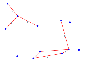
We can lay such a graph on the plane to visualise it, drawing only the finite edges:

The procedure can be explained as follows: we let a parameter $\varepsilon$ start at 0, and as we increase it all the way to infinity we keep considering the instantaneous subgraphs made of a) all the vertices in the original graph, and b) those edges whose weight is less than or equal to the current $\varepsilon$. We also promote these subgraphs to more general structures called (simplicial) complexes that, alongside vertices and edges, also possess $k$-simplices, i.e. selected subsets of $k + 1$ vertices (a 2-simplex is an abstract "triangle", a 3-simplex an abstract "tetrahedron", etc). Our criterion is this: for each integer $k \geq 2$, all $(k + 1)$-cliques in each instantaneous subgraph are declared to be the $k$-simplices of the subgraph's associated complex. By definition, the $0$-simplices are the vertices and the $1$-simplices are the available edges.
As $\varepsilon$ increases from 0 (included) to infinity, we record the following information:
- How many new connected components are created because of the appearance of vertices (in this example, all vertices "appear" in one go at $\varepsilon = 0$, by definition!), or merge because of the appearance of new edges.
- How many new 1-dimensional "holes", 2-dimensional "cavities", or more generally $d$-dimensional voids are created in the instantaneous complex. A hole, cavity, or $d$-dimensional void is such only if there is no collection of "triangles", "tetrahedra", or $(d + 1)$-simplices which the void is the "boundary" of. Note: Although the edges of a triangle alone "surround a hole", these cannot occur in our particular construction because the "filling" triangle is also declared present in the complex when all its edges are.
- How many $d$-dimensional voids which were present at earlier values of $\epsilon$ are "filled" by $(d + 1)$-simplices which just appear.
This process of recording the full topological history of the graph across all edge weights is called (Vietoris-Rips) persistent homology.
Let us start at $\varepsilon = 0$: Some edges had zero weight in our graph, so they already appear!

There are 9 connected components, and nothing much else.
Up to and including $\varepsilon = 2$, a few more edges are added which make some of the connected components merge together but do not create any hole, triangles, or higher cliques. Let us look at $\varepsilon = 3$:
The newly arrived edges reduce the number of connected components further, but more interestingly they create a 1D hole!
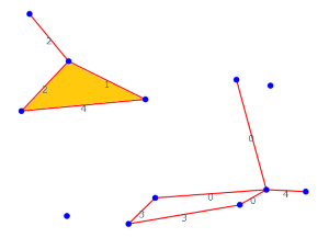
As an example of a "higher"-simplex, at $\varepsilon = 4$ we get our first triangle:
At $\varepsilon = 5$, our 1D hole is filled:

At $\varepsilon = 8$, two new 1D holes appear:

Finally, at $\varepsilon = 9$, some more connected components merge, but no new voids are either created or destroyed:
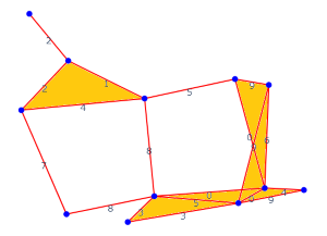
We can stop as we have reached the maximum value of $\varepsilon$, beyond which nothing will change: there is only one connected component left, but there are also two 1D holes which will never get filled.
Fit-transforming via VietorisRipsPersistence(metric="precomputed") on the original graph's adjacency matrix would return the following 3D array of persistence diagrams:
diagrams = np.array([[[0., 1., 0],
                      [0., 2., 0],
                      [0., 2., 0],
                      [0., 3., 0],
                      [0., 4., 0],
                      [0., 5., 0],
                      [0., 6., 0],
                      [0., 7., 0],
                      [3., 5., 1],
                      [8., np.inf, 1],
                      [8., np.inf, 1]]])
The notebook Topological feature extraction using VietorisRipsPersistence and PersistenceEntropy explains how to interpret this output and how to make informative 2D scatter plots out of its entries. Here, we only have one entry corresponding to our graph:
from gtda.plotting import plot_diagram

plot_diagram(diagrams[0])
Small aside: You would be correct to expect an additional row [0, np.inf, 0] representing one connected component which lives forever. By convention, since such a row would always be present under this construction and hence give no useful information, all transformers discussed in this notebook remove this feature from the output.
Advanced discussion: Non-zero vertex weights and negative edge weights
Although we introduced the simplifying assumptions that the diagonal entries of the input adjacency matrix is zero, and that all edge weights are non-negative, for the procedure to make sense we need a lot less. Namely:
- The diagonal entry corresponding to a vertex is always interpreted as the value of the parameter $\varepsilon$ at which that vertex "appears". Making all these entries equal to zero means, as in the example above, that all vertices appear simultaneously at $\varepsilon = 0$. Generally however, different vertices can be declared to "appear" at different values, and even at negative ones.
- The only constraint on each edge weight is that it should be no less than the "vertex weight" of either of its boundary vertices.
As a simple example, subtracting a constant from all entries of an adjacency matrix has the effect of shifting all birth and death values by the same constant.
The "special case" of point clouds
The use of VietorisRipsPersistence to compute multi-scale topological features of concrete point clouds in Euclidean space is covered briefly in Section 1.2 of Plotting in giotto-tda, and more in-depth in Classifying 3D shapes and in Can two-dimensional topological voids exist in two dimensions?
The Vietoris-Rips procedure for point clouds is often depicted as a process of growing balls of ever increasing radius $r$ around each point, and drawing edges between two points whenever their two respective $r$-balls touch for the first time. Just as in our clique complex construction above, cliques present at radius $r$ are declared to be higher-dimensional simplices in the instantaneous complex:
And just as in the case of weighted graphs, we record the appearance/disappearance of connected components and voids as we keep increasing $r$.
The case of point clouds can actually be thought of as a special case of the case of FCW graphs. Namely, if:
- we regard each point in the cloud as an abstract vertex in a graph,
- we compute the square matrix of pairwise (Euclidean or other) distances between points in the cloud, and
- we run the procedure explained above with $\varepsilon$ defined as $2r$,
then we compute exactly the "topological summary" of the point cloud.
So, in giotto-tda, we can do:
# 1 point cloud with 20 points in 5 dimensions
point_cloud = rng.random((20, 5))
# Corresponding matrix of Euclidean pairwise distances
pairwise_distances = squareform(pdist(point_cloud))

# Default parameter for ``metric`` is "euclidean"
X_vr_pc = VietorisRipsPersistence().fit_transform([point_cloud])

X_vr_graph = VietorisRipsPersistence(metric="precomputed").fit_transform([pairwise_distances])

assert np.array_equal(X_vr_pc, X_vr_graph)
Unweighted graphs and chaining with GraphGeodesicDistance
What if, as is the case in many applications, our graphs have sparse connections and are unweighted?
In giotto-tda, there are two possibilities:
- Encode the graphs as adjacency matrices of non-fully connected weighted graphs, where all weights corresponding to edges which are present are equal to
1.(or any other positive constant). See section *Non-fully connected weighted graphs* above for the different encoding conventions for sparse and dense matrices. - Preprocess the unweighted graph via GraphGeodesicDistance to obtain a FCW graph where edge $ij$ has as weight the length of the shortest path from vertex $i$ to vertex $j$ (and
np.infif no path exists between the two vertices in the original graph).
Example 1: Circle graph
We now explore the difference between the two approaches in the simple example of a circle graph.
# Helper function -- directed circles will be needed later
def make_circle_adjacency(n_vertices, directed=False):
    weights = np.ones(n_vertices)
    rows = np.arange(n_vertices)
    columns = np.arange(1, n_vertices + 1) % n_vertices
    directed_adjacency = csr_matrix((weights, (rows, columns)))
    if not directed:
        return directed_adjacency + directed_adjacency.T
    return directed_adjacency

n_vertices = 10
undirected_circle = make_circle_adjacency(n_vertices)
We can produce an SVG of the circle using python-igraph, and display it.
Note: If running from a live jupyter session, this will dump a file inside your notebook's directory. If pycairo is installed, you can draw the graph directly in the notebook by instead running
from igraph import plot
plot(graph)
in the cell below.
row, col = undirected_circle.nonzero()
graph = Graph(n=n_vertices, edges=list(zip(row, col)), directed=False)
fname = "undirected_circle.svg"
graph.write_svg(fname)
display(SVG(filename=fname))
Approach 1 means passing the graph as is:
VietorisRipsPersistence(metric="precomputed").fit_transform_plot([undirected_circle]);
The circular nature has been captured by the single point in homology dimension 1 ($H_1$) which is born at 1 and lives forever.
Compare with what we observe when preprocessing first with GraphGeodesicDistance:
X_ggd = GraphGeodesicDistance(directed=False, unweighted=True).fit_transform([undirected_circle])
VietorisRipsPersistence(metric="precomputed").fit_transform_plot(X_ggd);
There is still a "long-lived" topological feature in dimension 1, but this time its death value is finite. This is because, at some point, we have enough triangles to completely fill the 1D hole. Indeed, when the number of vertices/edges in the circle is large, the death value is around one third of this number. So, relative to the procedure without GraphGeodesicDistance, the death value now gives additional information about the size of the circle graph!
Example 2: Two disconnected circles
Suppose our graph contains two disconnected circles of different sizes:
n_vertices_small, n_vertices_large = n_vertices, 2 * n_vertices
undirected_circle_small = make_circle_adjacency(n_vertices_small)
undirected_circle_large = make_circle_adjacency(n_vertices_large)
row_small, col_small = undirected_circle_small.nonzero()
row_large, col_large = undirected_circle_large.nonzero()
row = np.concatenate([row_small, row_large + n_vertices])
col = np.concatenate([col_small, col_large + n_vertices])
data = np.concatenate([undirected_circle_small.data, undirected_circle_large.data])
two_undirected_circles = csr_matrix((data, (row, col)))

graph = Graph(n=n_vertices_small + n_vertices_large, edges=list(zip(row, col)), directed=False)
fname = "two_undirected_circles.svg"
graph.write_svg(fname)
display(SVG(filename=fname))
Again, the first procedure just says "there are two 1D holes".
VietorisRipsPersistence(metric="precomputed").fit_transform_plot([two_undirected_circles]);
The second procedure is again much more informative, yielding a persistence diagram with two points in homology dimension 1 with different finite deaths, each corresponding to one of the two circles:
X_ggd = GraphGeodesicDistance(directed=False, unweighted=True).fit_transform([two_undirected_circles])
VietorisRipsPersistence(metric="precomputed").fit_transform_plot(X_ggd);
Directed graphs – FlagserPersistence
Together with the companion package pyflagser (source code, API reference), giotto-tda can extract topological features from directed graphs via the FlagserPersistence transformer.
Unlike VietorisRipsPersistence and SparseRipsPersistence, FlagserPersistence only works on graph data, so there is no metric parameter to be set. The conventions on input data are the same as in the undirected case, cf. section *Non-fully connected weighted graphs* above.
The ideas and constructions underlying the algorithm in this case are very similar to the ones described above for the undirected case. Again, we threshold the graph and its directed edges according to an ever-increasing parameter and the edge weights. And again we look at "cliques" of vertices to define simplices and hence a "complex" for each value of the parameter. The main difference is that here simplices are ordered sets (tuples) of vertices, and that in each instantaneous complex the "clique" $(v_0, v_1, \ldots, v_k)$ is a $k$-simplex if and only if, for each $i < j$, $(v_i, v_j)$ is a currently present directed edge.
| (1, 2, 3) *is not* a 2-simplex in the complex | (1, 2, 3) *is* a 2-simplex in the complex |
|---|---|
 |
 |
| (1, 2), (2, 3) and (3, 1) form a 1D hole | (1, 2), (2, 3) and (1, 3) form the boundary of (1, 2, 3) – not a 1D hole |
This has interesting consequences: in the examples above, the left complex, in which the edges of the triangle "loop around" in the same direction, contains a 1D hole. On the other hand, the right one does not!
Example 1: Directed circle
Let's try this on a "directed" version of the circle from earlier:
n_vertices = 10

directed_circle = make_circle_adjacency(n_vertices, directed=True)
row, col = directed_circle.nonzero()

graph = Graph(n=n_vertices, edges=list(zip(row, col)), directed=True)
fname = "directed_circle.svg"
graph.write_svg(fname)
display(SVG(filename=fname))
Passing this directly to FlagserPersistence gives an unsurprising result:
FlagserPersistence().fit_transform_plot([directed_circle]);
Again, we can chain with an instance of GraphGeodesicDistance to get more information:
X_ggd = GraphGeodesicDistance(directed=True, unweighted=True).fit_transform([directed_circle])
FlagserPersistence().fit_transform_plot(X_ggd);
Notice that this time the death time of the circular feature is circa one half of the number of vertices/edges. Compare this with the one-third factor we observed in the case of VietorisRipsPersistence.
Example 2: Circle with alternating edge directions
What happens when we make some of the edges flow the other way around the circle?
row_flipped = np.concatenate([row[::2], col[1::2]])
column_flipped = np.concatenate([col[::2], row[1::2]])

graph = Graph(n=n_vertices, edges=list(zip(row_flipped, column_flipped)), directed=True)
fname = "directed_circle.svg"
graph.write_svg(fname)
display(SVG(filename=fname))
# Construct the adjacency matrix
weights = np.ones(n_vertices)
directed_circle_flipped = csr_matrix((weights, (row_flipped, column_flipped)),
                                     shape=(n_vertices, n_vertices))

# Run FlagserPersistence directly on the adjacency matrix
FlagserPersistence().fit_transform_plot([directed_circle_flipped]);
This is identical to the persistence diagram for the directed circle (and for the undirected circle using VietorisRipsPersistence). We cannot tell the difference between the two directed graphs when the adjacency matrices are fed directly to FlagserPersistence. Let's try with GraphGeodesicDistance:
X_ggd = GraphGeodesicDistance(directed=True, unweighted=True).fit_transform([directed_circle_flipped])
FlagserPersistence().fit_transform_plot(X_ggd);
As in the case of the directed circle, the one-dimensional feature is born at 1. However, unlike that case, it persists all the way to infinity even after preprocessing with GraphGeodesicDistance!
Example 3: Two oppositely-directed semicircles
Our final example consists of a circle one half of which "flows" in one direction, and the other half in the other.
row_two_semicircles = np.concatenate([row[:n_vertices // 2], col[n_vertices // 2:]])
column_two_semicircles = np.concatenate([col[:n_vertices // 2], row[n_vertices // 2:]])

graph = Graph(n=n_vertices, edges=list(zip(row_two_semicircles, column_two_semicircles)), directed=True)
fname = "two_directed_semicircles.svg"
graph.write_svg(fname)
display(SVG(filename=fname))
# Construct the adjacency matrix
weights = np.ones(n_vertices)
two_semicircles = csr_matrix((weights, (row_two_semicircles, column_two_semicircles)),
                             shape=(n_vertices, n_vertices))

# Run FlagserPersistence directly on the adjacency matrix
FlagserPersistence().fit_transform_plot([two_semicircles]);
Again, we passed the adjacency matrix directly and obtained the same persistence diagram as for the undirected circle. Let's try preprocessing with GraphGeodesicDistance:
X_ggd = GraphGeodesicDistance(directed=True, unweighted=True).fit_transform([two_semicircles])
FlagserPersistence(directed=True).fit_transform_plot(X_ggd);
This is similar to the persistence diagram for the coherently directed circle, but the death time for the topological feature in dimension 1 is slightly lower.
Where to next?
- Persistence diagrams are great for data exploration, but to feed their content to machine learning algorithms one must make sure the algorithm used is independent of the relative ordering of the birth-death pairs in each homology dimension. gtda.diagrams contains a suite of vector representations, feature extraction methods and kernel methods that convert persistence diagrams into data structures ready for machine learning algorithms. Simple examples of their use are contained in Topological feature extraction using VietorisRipsPersistence and PersistenceEntropy, Classifying 3D shapes and Lorenz attractor.
- In addition to
GraphGeodesicDistance, gtda.graphs also contains transformers for the creation of graphs from point cloud or time series data. - Despite the name, gtda.point_clouds contains transformers for the alteration of distance matrices (which are just adjacency matrices of weighted graphs) as a preprocessing step for persistent homology.
VietorisRipsPersistencebuilds on the ripser.py project. Its website contains two tutorials on additional ways in which graphs can be constructed from time series data or image data, and fed to the clique complex filtration construction. With a few simple modifications, the code can be adapted to the API ofVietorisRipsPersistence.