%pylab inline
Populating the interactive namespace from numpy and matplotlib
from __future__ import print_function
from deltasigma import *
from IPython.core.display import Image
# skip this, this is just to display nice tables.
from itertools import izip_longest
class Table(list):
    def _repr_html_(self):
        html = ["<table>"]
        for row in self:
            html.append("<tr>")
            for col in row:
                try:
                    float(col)
                    html.append("<td>%.6f</td>" % col)
                except(ValueError):
                    html.append("<td><b>%s</b></td>" % col)
            html.append("</tr>")
        html.append("</table>")
        return ''.join(html)
Modulator realization and dynamic range scaling - # demo3
In this ipython notebook, the following is demonstrated:
A 5th order delta sigma modulator is synthesized, with optimized zeros and an OSR equal to 42.
We then convert the synthesized NTF into
a,g,b,ccoefficients for theCRFBmodulator structure.The maxima for each state are evaluated.
The
ABCDmatrix is scaled so that the state maxima are less than the specified limit.The state maxima are re-evaluated and limit compliance is checked.
NOTE: This is an ipython port of dsdemo3.m, from the MATLAB Delta Sigma Toolbox, written by Richard Schreier.
Delta sigma modulator synthesis
order = 5
R = 42
opt = 1
H = synthesizeNTF(order, R, opt)
Let's inspect the NTF, printing out the transfer function and plotting poles and zeros with respect to the unit circle.
print(pretty_lti(H))
        (z^2 - 1.995z + 1) (z^2 - 1.998z + 1) (z - 1)
--------------------------------------------------------------
 (z^2 - 1.614z + 0.6657) (z^2 - 1.797z + 0.8552) (z - 0.7783)
figure(figsize=(10, 5))
plotPZ(H, showlist=True)
title('NTF');

Evaluation of the coefficients for a CRFB topology
The CRFB topology is depicted in the following diagram.
Image(url='http://python-deltasigma.readthedocs.org/en/latest/_images/CRFB.png', retina=True)
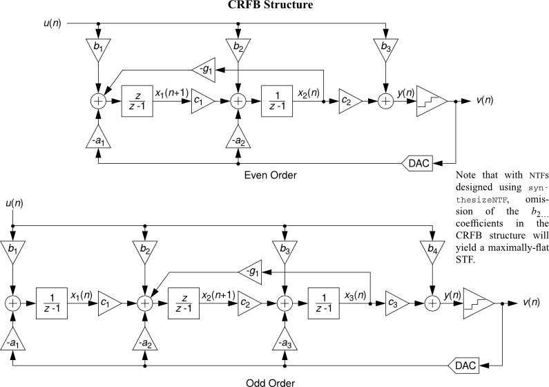
Since the modulator order is 5, we're interested in the topology for odd order modulators.
Unscaled modulator
Calculate the coefficients
a, g, b, c = realizeNTF(H)
Feed-in selection
We'll use a single feed-in for the input, to have a maximally flat STF.
This means setting $\ b_n = 0, \ \forall n > 1$.
b = np.concatenate((b[0].reshape((1, )), np.zeros((b.shape[0] - 1, ))), axis=0)
t = Table()
ilabels = ['#1', '#2', '#3', '#4', '#5', '#6']
t.append(['Coefficients', 'DAC feedback', 'Resonator feedback',
          'Feed-in', 'Interstage'])
t.append(['', 'a(n)', 'g(n)', ' b(n)', ' c(n)'])
[t.append(x) for x in izip_longest(ilabels, a.tolist(), g.tolist(), b.tolist(), c.tolist(), fillvalue="")]
t
| Coefficients | DAC feedback | Resonator feedback | Feed-in | Interstage |
| a(n) | g(n) | b(n) | c(n) | |
| #1 | 0.000667 | 0.001622 | 0.000667 | 1.000000 |
| #2 | 0.008583 | 0.004593 | 0.000000 | 1.000000 |
| #3 | 0.055201 | 0.000000 | 1.000000 | |
| #4 | 0.247607 | 0.000000 | 1.000000 | |
| #5 | 0.556935 | 0.000000 | 1.000000 | |
| #6 | 0.000000 |
Calculate the state maxima
ABCD = stuffABCD(a, g, b, c);
u = np.linspace(0, 0.6, 30);
N = 1e4;
T = np.ones((1, N))
maxima = np.zeros((order, len(u)))
for i in range(len(u)):
    ui = u[i]
    v, xn, xmax, _ = simulateDSM(ui*T, ABCD);
    maxima[:, i] = np.squeeze(xmax)
    if any(xmax > 1e2):
        umax = ui;
        u = u[:i+1];
        maxima = maxima[:, :i]
        break;
# save the maxima
prescale_maxima = np.copy(maxima)
print('The state maxima have been evaluated through simulation.')
The state maxima have been evaluated through simulation.
Plot of the state maxima
for i in range(order):
    semilogy(u, maxima[i, :],'o-')
    if not i:
        hold(True)
grid(True)
xlabel('DC input')
ylabel('Peak value')
title('Simulated State Maxima')
xlim([0, 0.6])
ylim([1e-4, 10]);

ABCDs, umax, _ = scaleABCD(ABCD, N_sim=1e5)
as_, gs, bs, cs = mapABCD(ABCDs)
print('\nScaled modulator, umax = %.2f\n' % umax)
Scaled modulator, umax = 0.58
t = Table()
ilabels = ['#1', '#2', '#3', '#4', '#5', '#6']
t.append(['Coefficients', 'DAC feedback', 'Resonator feedback',
          'Feed-in', 'Interstage'])
t.append(['', 'a(n)', 'g(n)', ' b(n)', ' c(n)'])
[t.append(x) for x in izip_longest(ilabels, as_.tolist(), gs.tolist(), bs.tolist(), cs.tolist(), fillvalue="")]
t
| Coefficients | DAC feedback | Resonator feedback | Feed-in | Interstage |
| a(n) | g(n) | b(n) | c(n) | |
| #1 | 0.100298 | 0.008508 | 0.100298 | 0.135347 |
| #2 | 0.174656 | 0.010817 | 0.000000 | 0.190649 |
| #3 | 0.214165 | 0.000000 | 0.380271 | |
| #4 | 0.365304 | 0.000000 | 0.424567 | |
| #5 | 0.348852 | 0.000000 | 1.596478 | |
| #6 | 0.000000 |
Calculate the state maxima
u = np.linspace(0, umax, 30)
N = 1e4
T = np.ones((N,))
maxima = np.zeros((order, len(u)))
for i in range(len(u)):
    ui = u[i]
    v, xn, xmax, _ = simulateDSM(ui*T, ABCDs)
    maxima[:, i] = xmax.squeeze()
    if any(xmax > 1e2):
        umax = ui;
        u = u[:i]
        maxima = maxima[:, :i]
        break
print('The state maxima have been re-evaluated through simulation.')
print("The maximum input was found to be %.6f" % umax)
The state maxima have been re-evaluated through simulation.
The maximum input was found to be 0.583333
Plot of the state maxima after scaling
for i in range(order):
    semilogy(u, maxima[i, :], 'o-')
    if not i:
        hold(True)
grid(True)
ylabel('Peak value')
xlabel('DC input')
xlim([0, 0.6])
ylim([4e-2, 4]);

System version information
#%install_ext http://raw.github.com/jrjohansson/version_information/master/version_information.py
%load_ext version_information
%reload_ext version_information

%version_information numpy, scipy, matplotlib, deltasigma
| Software | Version |
|---|---|
| Python | 2.7.5+ (default, Sep 17 2013, 17:31:54) [GCC 4.8.1] |
| IPython | 2.0.0 |
| OS | posix [linux2] |
| numpy | 1.8.0 |
| scipy | 0.13.0 |
| matplotlib | 1.3.1 |
| deltasigma | 0.1-1 |
| Tue Apr 29 20:25:29 2014 CEST | |