![]()
Introduction to Scikit-learn
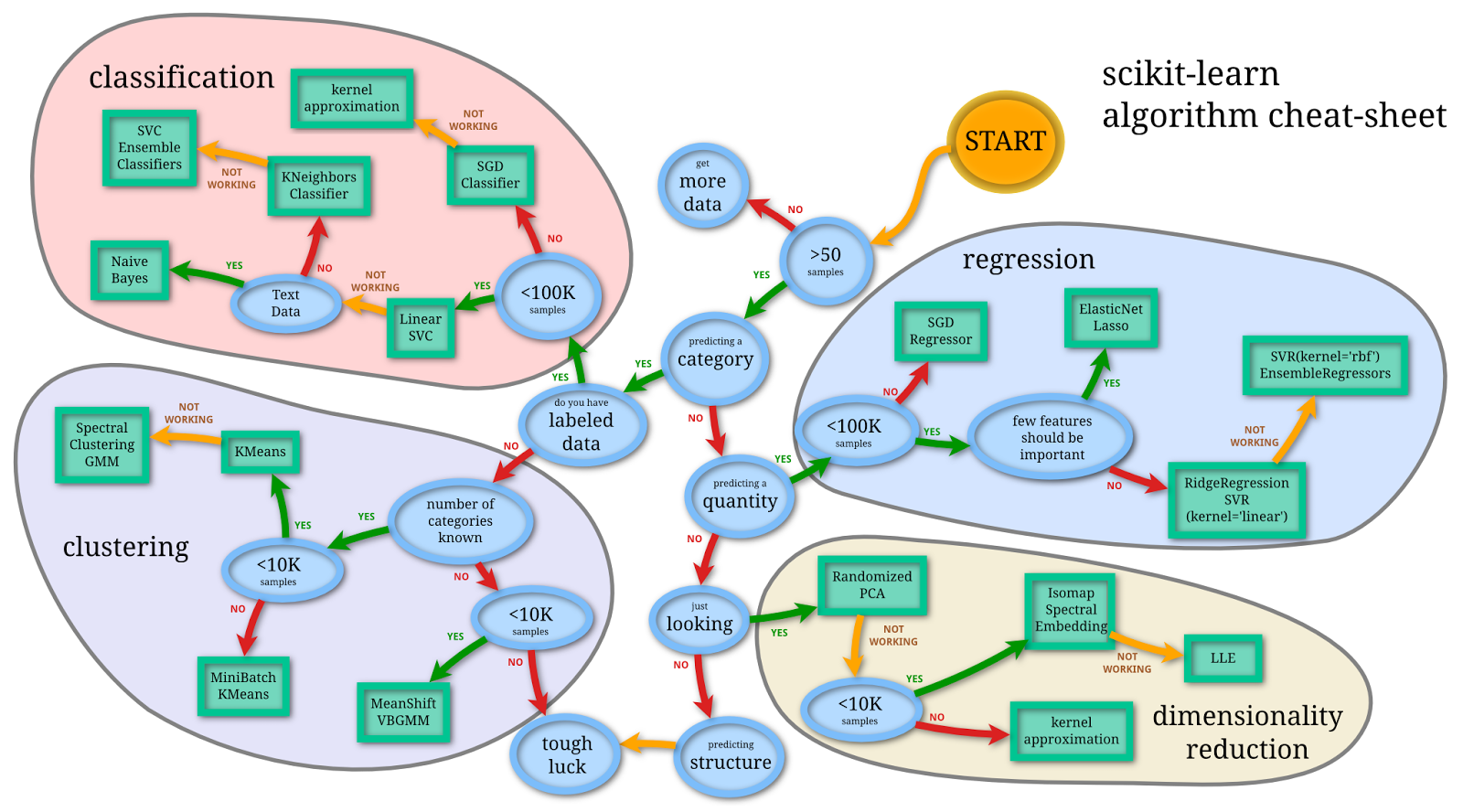
The scikit-learn package is an open-source library that provides a robust set of machine learning algorithms for Python. It is built upon the core Python scientific stack (i.e. NumPy, SciPy, Cython), and has a simple, consistent API, making it useful for a wide range of statistical learning applications.
What is Machine Learning?
Machine Learning (ML) is about coding programs that automatically adjust their performance from exposure to information encoded in data. This learning is achieved via tunable parameters that are automatically adjusted according to performance criteria.
Machine Learning can be considered a subfield of Artificial Intelligence (AI).
There are three major classes of ML:
- Supervised learning
- Algorithms which learn from a training set of labeled examples (exemplars) to generalize to the set of all possible inputs. Examples of supervised learning include regression and support vector machines.
- Unsupervised learning
- Algorithms which learn from a training set of unlableled examples, using the features of the inputs to categorize inputs together according to some statistical criteria. Examples of unsupervised learning include k-means clustering and kernel density estimation.
- Reinforcement learning
- Algorithms that learn via reinforcement from a critic that provides information on the quality of a solution, but not on how to improve it. Improved solutions are achieved by iteratively exploring the solution space. We will not cover RL in this course.
Representing Data in scikit-learn
Most machine learning algorithms implemented in scikit-learn expect data to be stored in a
two-dimensional array or matrix. The arrays can be
either numpy arrays, or in some cases scipy.sparse matrices.
The size of the array is expected to be [n_samples, n_features]
- n_samples: The number of samples: each sample is an item to process (e.g. classify). A sample can be a document, a picture, a sound, a video, an astronomical object, a row in database or CSV file, or whatever you can describe with a fixed set of quantitative traits.
- n_features: The number of features or distinct traits that can be used to describe each item in a quantitative manner. Features are generally real-valued, but may be boolean or discrete-valued in some cases.
The number of features must be fixed in advance. However it can be very high dimensional
(e.g. millions of features) with most of them being zeros for a given sample. This is a case
where scipy.sparse matrices can be useful, in that they are
much more memory-efficient than numpy arrays.
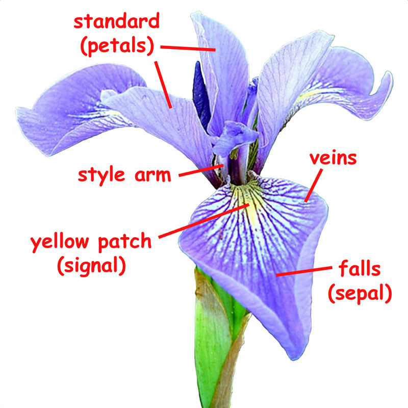
Example: Iris morphometrics
One of the datasets included with scikit-learn is a set of measurements for flowers, each being a member of one of three species: Iris Setosa, Iris Versicolor or Iris Virginica.
from sklearn.datasets import load_iris
iris = load_iris()
The data is stored as a dict with elements corresponding to the predictors (data), the species name (target), as well as labels associated with these values.
iris.keys()
n_samples, n_features = iris.data.shape
n_samples, n_features
Here is a sample row of the data, with the corresponding labels.
iris.data[0]
iris.feature_names
The information about the class of each sample is stored in the target attribute of the dataset:
iris.target
iris.target_names
We probably want to convert the data into a more convenient structure, namely, a DataFrame.
import pandas as pd

iris_df = pd.DataFrame(iris.data, columns=iris.feature_names).assign(species=iris.target_names[iris.target])

iris_df.head()
Principal Component Analysis
As an introductory application of machine learning methods, let's apply principal components analysis (PCA) to this dataset. Though we have 4 variables to work with, it appears that there is redundant information among them, so we might try to reduce the dimension of the problem, deriving a smaller number of latent variables that describe most of the overall variation in the dataset. For example, we might want 2 variables so that we can visualize differences among the species graphically.
PCA is a transformation for identifying a set of latent variables corresponding to orthogonal components of variation. It locates a vector that describes an axis of largest variation in the hyperspace of the original variables. Then, conditional on the first vector, the algorithm picks out the next vector of maximum variation, but one which is orthogonal to the first component. It then identifies a third such orthogonal vector, and so on, up to the number of original variables in the dataset.
Once we have this orthogonal set of variables, we can see if the smallest ones can be discarded without greatly reducing the amount of variation described by the remaining subset.
Here is an illustraion using the iris dataset.
import seaborn as sns

sns.pairplot(iris_df, hue='species', height=1.5);
We can see, for example, that the petal variables appear to be redundant with respect to one another.
What PCA will do is formulate a set of orthogonal varibles, where the number of orthogonal axes is smaller than the number of original variables. It then projects the original data onto these axes to obtain transformed variables.
The key concept is that each set of axes constructed maximizes the amount of residual variability explained.
We can then fit models to the subset of orthogonal variables that accounts for most of the variability.
Let's do a PCA by hand first, before using scikit-learn:
Standardization
An important first step for many datasets is to standardize the original data. Its important for all variables to be on the same scale because the PCA algorithm will be seeking to maximize variance along each axis. If one variable is numerically larger than another variable, it will tend to have larger variance, and will therefore garner undue attention from the algorithm.
This dataset is approximately on the same scale, though there are differences, particularly in the fourth variable (petal width):
iris.data[:5]
Let's apply a standardization transformation using the preprocessing capabilities of scikit-learn:
from sklearn.preprocessing import StandardScaler

X_std = StandardScaler().fit_transform(iris.data)
X_std[:5]
Eigendecomposition
The PCA algorithm is driven by the eigenvalues and eigenvectors of the original dataset.
- The eigenvectors determine the direction of each component
- The eigenvalues determine the length (magnitude) of the component
The eigendecomposition is performed on the covariance matrix of the data, which we can derive here using NumPy.
import numpy as np

Sigma = np.cov(X_std.T)
evals, evecs = np.linalg.eig(Sigma)
evals
import matplotlib.pyplot as plt
from mpl_toolkits.mplot3d import Axes3D
from mpl_toolkits.mplot3d import proj3d
from matplotlib.patches import FancyArrowPatch

variables = [name[:name.find(' (')]for name in iris.feature_names]

class Arrow3D(FancyArrowPatch):
    def __init__(self, xs, ys, zs, *args, **kwargs):
        FancyArrowPatch.__init__(self, (0,0), (0,0), *args, **kwargs)
        self._verts3d = xs, ys, zs

    def do_3d_projection(self, renderer=None):
        xs3d, ys3d, zs3d = self._verts3d
        xs, ys, zs = proj3d.proj_transform(xs3d, ys3d, zs3d, self.axes.M)
        self.set_positions((xs[0],ys[0]),(xs[1],ys[1]))

        return np.min(zs)

fig = plt.figure(figsize=(7,7))
ax = fig.add_subplot(111, projection='3d')

ax.plot(X_std[:,0], X_std[:,1], X_std[:,2], 'o', markersize=8,
        color='green',
        alpha=0.2)

mean_x, mean_y, mean_z = X_std.mean(0)[:-1]
ax.plot([mean_x], [mean_y], [mean_z], 'o', markersize=10, color='red', alpha=0.5)
for v in evecs:
    a = Arrow3D([mean_x, v[0]], [mean_y, v[1]], [mean_z, v[2]], mutation_scale=20, lw=3, arrowstyle="-|>", color="r")
    # ax.add_artist(a)
ax.set_xlabel(variables[0])
ax.set_ylabel(variables[1])
ax.set_zlabel(variables[2])

plt.title('Eigenvectors')
Selecting components
The eigenvectors are the principle components, which are normalized linear combinations of the original features. They are ordered, in terms of the amount of variation in the dataset that they account for.
fig, axes = plt.subplots(2, 1)

total = evals.sum()
variance_explained = 100* np.sort(evals)[::-1]/total

axes[0].bar(range(4), variance_explained)
axes[0].set_xticks(range(4));
axes[0].set_xticklabels(['Component ' + str(i+1) for i in range(4)])

axes[1].plot(range(5), np.r_[0, variance_explained.cumsum()])
axes[1].set_xticks(range(5));
Projecting the data
The next step is to project the original data onto the orthogonal axes.
Let's extract the first two eigenvectors and use them as the projection matrix for the original (standardized) variables.
W = evecs[:, :2]
Y = X_std @ W
df_proj = pd.DataFrame(np.hstack((Y, iris.target.astype(int).reshape(-1, 1))),
                      columns=['Component 1', 'Component 2', 'Species'])
sns.lmplot(x='Component 1', y='Component 2',
          data=df_proj,
          fit_reg=False,
          hue='Species');
The PCA procedure is implemented in scikit-learn in its decompoisition library:
from sklearn.decomposition import PCA

pca = PCA(n_components=2, whiten=True).fit(iris.data)
X_pca = pca.transform(iris.data)
By convention, scikit-learn exposes values estimated or calculated by its methods as public attributes on the model itself, with names appended with an underscore.
Inspecting the explained_variance_ratio_ attribute for our model, we see that the first two components explain more than 97% of the variation in the dataset.
pca.explained_variance_ratio_
iris_df['First Component'] = X_pca[:, 0]
iris_df['Second Component'] = X_pca[:, 1]

sns.lmplot(x='First Component', y='Second Component',
           data=iris_df,
           fit_reg=False,
           hue="species");
scikit-learn interface
All objects within scikit-learn share a uniform common basic API consisting of three complementary interfaces:
- estimator interface for building and fitting models
- predictor interface for making predictions
- transformer interface for converting data.
The estimator interface is at the core of the library. It defines instantiation mechanisms of objects and exposes a fit method for learning a model from training data. All supervised and unsupervised learning algorithms (e.g., for classification, regression or clustering) are offered as objects implementing this interface. Machine learning tasks like feature extraction, feature selection or dimensionality reduction are also provided as estimators.
The consistent interface across machine learning methods makes it easy to switch between different approaches without drastically changing the form of the data or the supporting code, making experimentation and prototyping fast and easy.
Scikit-learn strives to have a uniform interface across all methods. For example, a typical estimator follows this template:
class Estimator(object):

    def fit(self, X, y=None):
        """Fit model to data X (and y)"""
        self.some_attribute = self.some_fitting_method(X, y)
        return self

    def predict(self, X_test):
        """Make prediction based on passed features"""
        pred = self.make_prediction(X_test)
        return pred
For a given scikit-learn estimator object (let's call it model), several methods are available. Irrespective of the type of estimator, there will be a fit method:
model.fit: fit training data. For supervised learning applications, this accepts two arguments: the dataXand the labelsy(e.g.model.fit(X, y)). For unsupervised learning applications, this accepts only a single argument, the dataX(e.g.model.fit(X)).
During the fitting process, the state of the estimator is stored in attributes of the estimator instance named with a trailing underscore character (_). For example, the sequence of regression trees
sklearn.tree.DecisionTreeRegressoris stored inestimators_attribute.
The predictor interface extends the notion of an estimator by adding a predict method that takes an array X_test and produces predictions based on the learned parameters of the estimator. In the case of supervised learning estimators, this method typically returns the predicted labels or values computed by the model. Some unsupervised learning estimators may also implement the predict interface, such as k-means, where the predicted values are the cluster labels.
supervised estimators are expected to have the following methods:
model.predict: given a trained model, predict the label of a new set of data. This method accepts one argument, the new dataX_new(e.g.model.predict(X_new)), and returns the learned label for each object in the array.model.predict_proba: For classification problems, some estimators also provide this method, which returns the probability that a new observation has each categorical label. In this case, the label with the highest probability is returned bymodel.predict().model.score: for classification or regression problems, most (all?) estimators implement a score method. Scores are between 0 and 1, with a larger score indicating a better fit.
Since it is common to modify or filter data before feeding it to a learning algorithm, some estimators in the library implement a transformer interface which defines a transform method. It takes as input some new data X_test and yields as output a transformed version. Preprocessing, feature selection, feature extraction and dimensionality reduction algorithms are all provided as transformers within the library.
unsupervised estimators will always have these methods:
model.transform: given an unsupervised model, transform new data into the new basis. This also accepts one argumentX_new, and returns the new representation of the data based on the unsupervised model.model.fit_transform: some estimators implement this method, which more efficiently performs a fit and a transform on the same input data.
Regression Analysis
To demonstrate how scikit-learn is used, let's conduct a logistic regression analysis on a dataset for very low birth weight (VLBW) infants.
Data on 671 infants with very low (less than 1600 grams) birth weight from 1981-87 were collected at Duke University Medical Center by OShea et al. (1992). Of interest is the relationship between the outcome intra-ventricular hemorrhage and the predictors birth weight, gestational age, presence of pneumothorax, mode of delivery, single vs. multiple birth, and whether the birth occurred at Duke or at another hospital with later transfer to Duke. A secular trend in the outcome is also of interest.
The metadata for this dataset can be found here.
DATA_URL = 'https://raw.githubusercontent.com/fonnesbeck/Bios8366/master/data/'

try:
    vlbw = pd.read_csv("../data/vlbw.csv", index_col=0)
except FileNotFoundError:
    vlbw = pd.read_csv(DATA_URL + "vlbw.csv", index_col=0)


subset = vlbw[['ivh', 'gest', 'bwt', 'delivery', 'inout',
               'pltct', 'lowph', 'pneumo', 'twn', 'apg1']].dropna()

# Extract response variable
y = subset.ivh.replace({'absent':0, 'possible':1, 'definite':1})

# Standardize some variables
X = subset[['gest', 'bwt', 'pltct', 'lowph']]
X0 = (X - X.mean(axis=0)) / X.std(axis=0)

# Recode some variables
X0['csection'] = subset.delivery.replace({'vaginal':0, 'abdominal':1})
X0['transported'] = subset.inout.replace({'born at Duke':0, 'transported':1})
X0[['pneumo', 'twn', 'apg1']] = subset[['pneumo', 'twn','apg1']]
X0.head()
We first split the data into a training set and a testing set. By default, 25% of the data is reserved for testing. This is the first of multiple ways that we will see to do this.
from sklearn.model_selection import train_test_split
X_train, X_test, y_train, y_test = train_test_split(X0, y)
The LogisticRegression model in scikit-learn employs a regularization coefficient C, which defaults to 1. The amount of regularization is lower with larger values of C.
Regularization penalizes the values of regression coefficients, while smaller ones let the coefficients range widely. Scikit-learn includes two penalties: a l2 penalty which penalizes the sum of the squares of the coefficients (the default), and a l1 penalty which penalizes the sum of the absolute values.
The reason for doing regularization is to let us to include more covariates than our data might otherwise allow. We only have a few coefficients, so we will set C to a large value.
from sklearn.linear_model import LogisticRegression

lrmod = LogisticRegression(C=1000, solver='lbfgs')
lrmod
The __repr__ method of scikit-learn models prints out all of the hyperparameter values used when running the model. It is recommended to inspect these prior to running the model, as the can strongly influence the resulting estimates and predictions.
lrmod.fit(X_train, y_train)

pred_train = lrmod.predict(X_train)
pred_test = lrmod.predict(X_test)
pd.crosstab(y_train, pred_train,
            rownames=["Actual"], colnames=["Predicted"])
pd.crosstab(y_test, pred_test,
            rownames=["Actual"], colnames=["Predicted"])
The regression coefficients can be inspected in the coef_ attribute that the fitting procedure attached to the model object.
for name, value in zip(X0.columns, lrmod.coef_[0]):
    print('{0}:\t{1:.2f}'.format(name, value))
scikit-learn does not calculate confidence intervals for the model coefficients, but we can bootstrap some in just a few lines of Python:
import numpy as np

n = 1000
boot_samples = np.empty((n, len(lrmod.coef_[0])))

for i in np.arange(n):
    boot_ind = np.random.randint(0, len(X0), len(X0))
    y_i, X_i = y.values[boot_ind], X0.values[boot_ind]

    lrmod_i = LogisticRegression(C=1000, solver='lbfgs')
    lrmod_i.fit(X_i, y_i)

    boot_samples[i] = lrmod_i.coef_[0]
boot_samples.sort(axis=0)
boot_se = boot_samples[[25, 975], :].T
import matplotlib.pyplot as plt

coefs = lrmod.coef_[0]
plt.plot(coefs, 'r.')
for i in range(len(coefs)):
    plt.errorbar(x=[i,i], y=boot_se[i], color='red')
plt.xlim(-0.5, 8.5)
plt.xticks(range(len(coefs)), X0.columns.values, rotation=45)
plt.axhline(0, color='k', linestyle='--')
References
scikit-learnuser's guide- Vanderplas, J. (2016) Python Data Science Handbook: Essential Tools for Working with Data. O'Reilly Media.