エンコーダ用の階層型データ(vim-2)
ここでは2種類のデータを扱うことになる。視覚刺激としての自然動画像と、fMRIで測定したBOLD信号(血中酸素濃度に依存する信号)の2種類である。前者はいわば「入力」で、後者は脳活動の指標で、「応答」である。
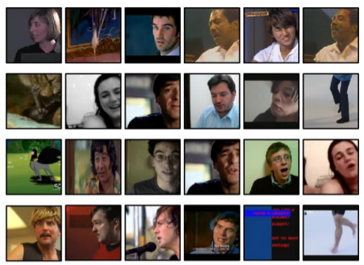
主要の目的として、入力画像から脳活動を正確に予測することを掲げる。イメージとして、画像を応答信号へと「符号化」していることから、このシステムを「エンコーダ」と呼ぶことが多い。
データセットの概要
今回使うデータの名称は「Gallant Lab Natural Movie 4T fMRI Data set」で、通称はvim-2である。その中身を眺めてみると:
視覚刺激
Stimuli.tar.gz 4089110463 (3.8 GB)
BOLD信号
VoxelResponses_subject1.tar.gz 3178624411 (2.9 GB)
VoxelResponses_subject2.tar.gz 3121761551 (2.9 GB)
VoxelResponses_subject3.tar.gz 3216874972 (2.9 GB)
視覚刺激はすべてStimuli.matというファイルに格納されている(形式:Matlab v.7.3)。その中身は訓練・検証データから構成される。
st: training stimuli. 128x128x3x108000 matrix (108000 128x128 rgb frames).sv: validation stimuli. 128x128x3x8100 matrix (8100 128x128 rgb frames).
訓練データに関しては、視覚刺激は15fpsで120分間提示されたため、7200の時点で合計108000枚のフレームから成る。検証データについては、同様に15fpsで9分間提示されたため、540の時点で合計8100枚のフレームから成る。検証用の視覚刺激は10回被験者に提示されたが、今回使う応答信号は、その10回の試行から算出した平均値である。平均を取る前の「生」データは公開されているが、ここでは使わない。
あと、データを並べ替える必要は特にない。作者の説明:
"The order of the stimuli in the "st" and "sv" variables matches the order of the stimuli in the "rt" and "rv" variables in the response files."
前へ進むには、これらのファイルを解凍しておく必要がある。
$ tar -xzf Stimuli.tar.gz
$ tar -xzf VoxelResponses_subject1.tar.gz
$ tar -xzf VoxelResponses_subject2.tar.gz
$ tar -xzf VoxelResponses_subject3.tar.gz
するとStimuli.matおよびVoxelResponses_subject{1,2,3}.matが得られる。階層的な構造を持つデータなので、開閉、読み書き、編集等を楽にしてくれるPyTables( http://www.pytables.org/usersguide/index.html )というライブラリを使う。シェルからファイルの中身とドキュメンテーションを照らし合わせてみると、下記のような結果が出てくる。
$ ptdump Stimuli.mat
/ (RootGroup) ''
/st (EArray(108000, 3, 128, 128), zlib(3)) ''
/sv (EArray(8100, 3, 128, 128), zlib(3)) ''
かなり単純な「階層」ではあるが、RootGroupにはフォルダー(stとsv)が2つある。それぞれの座標軸の意味を確認すると、1つ目は時点、2つ目は色チャネル(RGB)、3つ目と4つ目のペアは2次元配列における位置を示す。
次に応答信号のデータに注視すると、もう少し豊かな階層構造が窺える。
$ ptdump VoxelResponses_subject1.mat
/ (RootGroup) ''
/rt (EArray(73728, 7200), zlib(3)) ''
/rv (EArray(73728, 540), zlib(3)) ''
/rva (EArray(73728, 10, 540), zlib(3)) ''
(...Warnings...)
/ei (Group) ''
/ei/TRsec (Array(1, 1)) ''
/ei/datasize (Array(3, 1)) ''
/ei/imhz (Array(1, 1)) ''
/ei/valrepnum (Array(1, 1)) ''
/roi (Group) ''
/roi/FFAlh (EArray(18, 64, 64), zlib(3)) ''
/roi/FFArh (EArray(18, 64, 64), zlib(3)) ''
/roi/IPlh (EArray(18, 64, 64), zlib(3)) ''
/roi/IPrh (EArray(18, 64, 64), zlib(3)) ''
/roi/MTlh (EArray(18, 64, 64), zlib(3)) ''
/roi/MTplh (EArray(18, 64, 64), zlib(3)) ''
/roi/MTprh (EArray(18, 64, 64), zlib(3)) ''
/roi/MTrh (EArray(18, 64, 64), zlib(3)) ''
/roi/OBJlh (EArray(18, 64, 64), zlib(3)) ''
/roi/OBJrh (EArray(18, 64, 64), zlib(3)) ''
/roi/PPAlh (EArray(18, 64, 64), zlib(3)) ''
/roi/PPArh (EArray(18, 64, 64), zlib(3)) ''
/roi/RSCrh (EArray(18, 64, 64), zlib(3)) ''
/roi/STSrh (EArray(18, 64, 64), zlib(3)) ''
/roi/VOlh (EArray(18, 64, 64), zlib(3)) ''
/roi/VOrh (EArray(18, 64, 64), zlib(3)) ''
/roi/latocclh (EArray(18, 64, 64), zlib(3)) ''
/roi/latoccrh (EArray(18, 64, 64), zlib(3)) ''
/roi/v1lh (EArray(18, 64, 64), zlib(3)) ''
/roi/v1rh (EArray(18, 64, 64), zlib(3)) ''
/roi/v2lh (EArray(18, 64, 64), zlib(3)) ''
/roi/v2rh (EArray(18, 64, 64), zlib(3)) ''
/roi/v3alh (EArray(18, 64, 64), zlib(3)) ''
/roi/v3arh (EArray(18, 64, 64), zlib(3)) ''
/roi/v3blh (EArray(18, 64, 64), zlib(3)) ''
/roi/v3brh (EArray(18, 64, 64), zlib(3)) ''
/roi/v3lh (EArray(18, 64, 64), zlib(3)) ''
/roi/v3rh (EArray(18, 64, 64), zlib(3)) ''
/roi/v4lh (EArray(18, 64, 64), zlib(3)) ''
/roi/v4rh (EArray(18, 64, 64), zlib(3)) ''
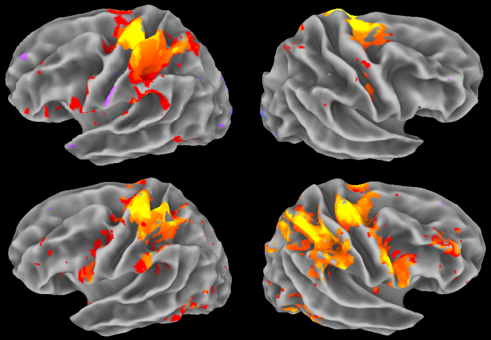
応答のデータでは、RootGroupのなかには、まずrt、rv、rvaという3つの配列がある。これらはBOLD信号の測定値を格納している。また、roiとeiと名付けられたgroupがある。前者は応答信号の時系列とボクセルを結びつけるためのインデックスである。後者は実験の条件等を示す数値が格納されている。ここでroiのほうに注目すると、計測された脳の領域全体を分割して(構成要素:ボクセル)、それを生理的・解剖学的に関心を持つべき「関心領域」(ROI)に振り分けていくのだが、このroiなるグループは、各ROIの名が付いた配列を含む。たとえば、v4rhとは__V4__という領域で、左半球(__l__eft __h__emisphere)に限定したROIのことである。明らかなように、ROIの数はボクセル数($18 \times 64 \times 64 = 73728$)よりも遥かに少ないので、各ROIが多数のボクセルを含むことがわかる。
import numpy as np
import tables
import matplotlib
from matplotlib import pyplot as plt
import pprint as pp

# Open file connection.
f = tables.open_file("data/vim-2/Stimuli.mat", mode="r")

# Get object and array.
stimulus_object = f.get_node(where="/", name="st")
print("stimulus_object:")
print(stimulus_object)
print(type(stimulus_object))
print("----")

stimulus_array = stimulus_object.read()
print("stimulus_array:")
#print(stimulus_array)
print(type(stimulus_array))
print("----")

# Close the connection.
f.close()

# Check that it is closed.
if not f.isopen:
    print("Successfully closed.")
else:
    print("File connection is still open.")
stimulus_object:
/st (EArray(108000, 3, 128, 128), zlib(3)) ''
<class 'tables.earray.EArray'>
----
stimulus_array:
<class 'numpy.ndarray'>
----
Successfully closed.
指定した配列の中身が予想通りのものを格納していること、正しく読み込めていることなどを確かめる必要がある。
# Open file connection.
f = tables.open_file("data/vim-2/Stimuli.mat", mode="r")
# Get object and array.
stimulus_object = f.get_node(where="/", name="st")
print("stimulus_object:")
print(stimulus_object)
print(type(stimulus_object))
print("----")
stimulus_object:
/st (EArray(108000, 3, 128, 128), zlib(3)) ''
<class 'tables.earray.EArray'>
----
# Print out basic attributes.
stimulus_array = stimulus_object.read()
#print("stimulus_array:")
#print(stimulus_array)
print("(type)")
print(type(stimulus_array))
print("(dtype)")
print(stimulus_array.dtype)
print("----")
(type)
<class 'numpy.ndarray'>
(dtype)
uint8
----
# Print out some frames.
num_frames = stimulus_array.shape[0]
num_channels = stimulus_array.shape[1]
frame_w = stimulus_array.shape[2]
frame_h = stimulus_array.shape[3]

frames_to_play = 5

oneframe = np.zeros(num_channels*frame_h*frame_w, dtype=np.uint8).reshape((frame_h, frame_w, num_channels))
im = plt.imshow(oneframe)

for t in range(frames_to_play):
    oneframe[:,:,0] = stimulus_array[t,0,:,:] # red
    oneframe[:,:,1] = stimulus_array[t,1,:,:] # green
    oneframe[:,:,2] = stimulus_array[t,2,:,:] # blue
    plt.imshow(oneframe)
    plt.show()


# Close file connection.
f.close()
十分なフレーム数を重ねてみると、読み込んだデータが確かに動画像であることが確認できた。但し、向きがおかしいことと、フレームレートがかなり高いこと、この2点は後ほど対応する。
練習問題:
座標軸を適当に入れ替えて(
help(np.swapaxes)を参照)、動画の向きを修正してみてください。上では最初の数枚のフレームを取り出して確認したのだが、次は最後の数枚のフレームを確認しておくこと。
上記は検証データであったが、同様な操作(取り出して可視化すること)を訓練データ
stに対しても行うこと。上記の操作で、最初の100枚のフレームを取り出してください。フレームレートが15fpsなので、7秒弱の提示時間に相当する。上記のコードの
forループに着目し、rangeに代わって適当にnp.arangeを使うことで、時間的なダウンサンプリングが容易にできる。15枚につき1枚だけ取り出して、1fpsに変えてから、最初の100枚を見て、変更前との違いを確認してください。
入力パターン(視覚刺激):空間的ダウンサンプリング
画素数が多すぎると、後の計算が大変になるので、空間的なダウンサンプリング、つまり画像を縮小することが多い。色々なやり方はあるが、ここでは__scikit-image__というライブラリのtransformモジュールから、resizeという関数を使う。まずは動作確認。
from skimage import transform
from matplotlib import pyplot as plt
import imageio
import tables
import numpy as np

im = imageio.imread("img/bishop.png") # a 128px x 128px image
med_h = 96 # desired height in pixels
med_w = 96 # desired width in pixels
im_med = transform.resize(image=im, output_shape=(med_h,med_w), mode="reflect")

small_h = 32
small_w = 32
im_small = transform.resize(image=im, output_shape=(small_h,small_w), mode="reflect")

tiny_h = 16
tiny_w = 16
im_tiny = transform.resize(image=im, output_shape=(tiny_h,tiny_w), mode="reflect")
myfig = plt.figure(figsize=(18,4))

ax_im = myfig.add_subplot(1,4,1)
plt.imshow(im)
plt.title("Original image")
ax_med = myfig.add_subplot(1,4,2)
plt.imshow(im_med)
plt.title("Resized image (Medium)")
ax_small = myfig.add_subplot(1,4,3)
plt.imshow(im_small)
plt.title("Resized image (Small)")
ax_small = myfig.add_subplot(1,4,4)
plt.imshow(im_tiny)
plt.title("Resized image (Tiny)")

plt.show()

予想するように動いているようなので、視覚刺激の全フレームに対して同様な操作を行う。
# Open file connection.
f = tables.open_file("data/vim-2/Stimuli.mat", mode="r")
# Specify which subset to use.
touse_subset = "sv"
# Get object, array, and properties.
stimulus_object = f.get_node(where="/", name=touse_subset)
stimulus_array = stimulus_object.read()
num_frames = stimulus_array.shape[0]
num_channels = stimulus_array.shape[1]
# Swap the axes.
print("Stimulus array (before):", stimulus_array.shape)
stimulus_array = np.swapaxes(a=stimulus_array, axis1=0, axis2=3)
stimulus_array = np.swapaxes(a=stimulus_array, axis1=1, axis2=2)
print("Stimulus array (after):", stimulus_array.shape)
Stimulus array (before): (8100, 3, 128, 128)
Stimulus array (after): (128, 128, 3, 8100)
# Prepare new array of downsampled stimulus.
ds_h = 64
ds_w = 64

new_array = np.zeros(num_frames*num_channels*ds_h*ds_w, dtype=np.float32)
new_array = new_array.reshape((ds_h, ds_w, num_channels, num_frames))
# Iterate over frames to be resized.
for t in range(num_frames):
    new_array[:,:,:,t] = transform.resize(image=stimulus_array[:,:,:,t],
                                          output_shape=(ds_h,ds_w),
                                          mode="reflect")
    if t % 1000 == 0:
        print("Update: t =", t)

f.close()
Update: t = 0
Update: t = 1000
Update: t = 2000
Update: t = 3000
Update: t = 4000
Update: t = 5000
Update: t = 6000
Update: t = 7000
Update: t = 8000
ここで一つ注意すべきことは、縮小したあとの画像は、$\{0,1,\ldots,255\}$ではなく、$[0,1]$の実数値を取ることである。そのため、dtypeをnp.float32に変えている。
print("(Pre-downsize) max:", np.max(stimulus_array),
      "min:", np.min(stimulus_array),
      "ave:", np.mean(stimulus_array))
print("(Post-downsize) max:", np.max(new_array),
      "min:", np.min(new_array),
      "ave:", np.mean(new_array))
(Pre-downsize) max: 255 min: 0 ave: 90.50942391854745
(Post-downsize) max: 1.0 min: 0.0 ave: 0.3549391
バイナリ形式にして、ディスクに保存しておくことにする(PyTablesと比べて、速いかどうかは各自で試すと良い)。
fname = "data/vim-2/" + str(touse_subset) + "_downsampled.dat"
with open(fname, mode="bw") as fbin:
    new_array.tofile(fbin)

fname = "data/vim-2/" + str(touse_subset) + "_downsampled.info"
with open(fname, mode="w") as f:
    f.write("dtype: "+str(new_array.dtype)+"\n")
    f.write("shape: "+str(new_array.shape)+"\n")
練習問題:
上記の空間的ダウンサンプリングを訓練データ(
st)に対しても行なうこと。さらに思い切ったダウンサンプリングを試してみること。32x32、16x16などと小さくすることで、どのような利点があると思われるか。デメリットはどのようなものがあるか。
期待通りに作動しているかどうか確認するために、先ほど保存したファイルを読み込み、その中身を確かめる。まず、保存したデータの寸法を読み込む:
! cat data/vim-2/st_downsampled.info
! cat data/vim-2/sv_downsampled.info
dtype: float32
shape: (64, 64, 3, 108000)
dtype: float32
shape: (64, 64, 3, 8100)
これらの値を下記のように使うと、確かに期待通りのデータが保存されていることがわかる。
print("Training data:")
fname = "data/vim-2/" + "st" + "_downsampled.dat"
with open(fname, mode="br") as fbin:

    # Read array.
    arr_tocheck = np.fromfile(file=fbin, dtype=np.float32).reshape((64, 64, 3, 108000))

    # Check a few frames.
    num_frames = arr_tocheck.shape[3]
    frames_to_play = 10
    for t in np.arange(0, frames_to_play*15, 15):
        plt.imshow(arr_tocheck[:,:,:,t])
        plt.show()
Training data:


print("Testing data:")
fname = "data/vim-2/" + "sv" + "_downsampled.dat"
with open(fname, mode="br") as fbin:

    # Read array.
    arr_tocheck = np.fromfile(file=fbin, dtype=np.float32).reshape((64, 64, 3, 8100))

    # Check a few frames.
    num_frames = arr_tocheck.shape[3]
    frames_to_play = 10
    for t in np.arange(0, frames_to_play*15, 15):
        plt.imshow(arr_tocheck[:,:,:,t])
        plt.show()
Testing data:


import tables
import numpy as np

# Open file connection, writing new file to disk.
myh5 = tables.open_file("data/vim-2/stimulus_ds.h5",
                        mode="w",
                        title="vim-2: stimulus")
print(myh5)
data/vim-2/stimulus_ds.h5 (File) 'vim-2: stimulus'
Last modif.: 'Tue Mar 27 21:14:24 2018'
Object Tree:
/ (RootGroup) 'vim-2: stimulus'
# Load up our downsampled stimulus (training).
fname = "data/vim-2/" + "st" + "_downsampled.dat"
with open(fname, mode="br") as fbin:
    arr = np.fromfile(file=fbin, dtype=np.float32).reshape((64, 64, 3, 108000))

myh5.create_array(where=myh5.root, name="train", obj=arr, title="Training data")
print(myh5)
data/vim-2/stimulus_ds.h5 (File) 'vim-2: stimulus'
Last modif.: 'Tue Mar 27 21:14:34 2018'
Object Tree:
/ (RootGroup) 'vim-2: stimulus'
/train (Array(64, 64, 3, 108000)) 'Training data'
# Load up our downsampled stimulus (testing).
fname = "data/vim-2/" + "sv" + "_downsampled.dat"
with open(fname, mode="br") as fbin:
    arr = np.fromfile(file=fbin, dtype=np.float32).reshape((64, 64, 3, 8100))

myh5.create_array(where=myh5.root, name="test", obj=arr, title="Testing data")
print(myh5)
data/vim-2/stimulus_ds.h5 (File) 'vim-2: stimulus'
Last modif.: 'Tue Mar 27 21:14:42 2018'
Object Tree:
/ (RootGroup) 'vim-2: stimulus'
/test (Array(64, 64, 3, 8100)) 'Testing data'
/train (Array(64, 64, 3, 108000)) 'Training data'
myh5.close()
print(myh5)
<closed File>
バイナリー形式で保存したときと同様に、期待通りの中身があることを確かめておく。前者は読む速度が早いのですが、後者は使い勝手がきわめて良いので、階層型の形式を中心に今後の学習課題などを進めていく。
myh5 = tables.open_file("data/vim-2/stimulus_ds.h5", mode="r")
print(myh5)
myh5.close()
data/vim-2/stimulus_ds.h5 (File) 'vim-2: stimulus'
Last modif.: 'Tue Mar 27 21:14:47 2018'
Object Tree:
/ (RootGroup) 'vim-2: stimulus'
/test (Array(64, 64, 3, 8100)) 'Testing data'
/train (Array(64, 64, 3, 108000)) 'Training data'
# Check the training data.
myh5 = tables.open_file("data/vim-2/stimulus_ds.h5", mode="r")
arrInst = myh5.get_node(myh5.root, "train")
print(arrInst)
print(type(arrInst))
frames_to_play = 10
idx = np.arange(0, frames_to_play*15, 15)
arr = arrInst[:,:,:,idx]
print(arr.shape)
for t in range(arr.shape[3]):
    plt.imshow(arr[:,:,:,t])
    plt.show()
myh5.close()
/train (Array(64, 64, 3, 108000)) 'Training data'
<class 'tables.array.Array'>
(64, 64, 3, 10)
# Check the testing data.
myh5 = tables.open_file("data/vim-2/stimulus_ds.h5", mode="r")
arrInst = myh5.get_node(myh5.root, "test")
print(arrInst)
print(type(arrInst))
frames_to_play = 10
idx = np.arange(0, frames_to_play*15, 15)
arr = arrInst[:,:,:,idx]
print(arr.shape)
for t in range(arr.shape[3]):
    plt.imshow(arr[:,:,:,t])
    plt.show()
myh5.close()
/test (Array(64, 64, 3, 8100)) 'Testing data'
<class 'tables.array.Array'>
(64, 64, 3, 10)
PyTablesなるモジュールの代表的なクラスについて何点か:
Arrayはデータの形式がすべて同一であることが条件。また、逐次的にデータを追加することができない。EArrayは同様にデータの形式が同一であり、次元数も固定だが、自由にデータを追加することができる。Tableはデータの追加も、多種の形式も可能である。
我々としては、浮動小数点型で統一して、追加も特に必要ないので、基本的にArrayを用いることにする。
import numpy as np
import tables
import matplotlib
from matplotlib import pyplot as plt
import pprint as pp

# Open file connection.
f = tables.open_file("data/vim-2/VoxelResponses_subject1.mat", mode="r")
print(f)
data/vim-2/VoxelResponses_subject1.mat (File) ''
Last modif.: 'Tue Apr  1 05:55:05 2014'
Object Tree:
/ (RootGroup) ''
/rt (EArray(73728, 7200), zlib(3)) ''
/rv (EArray(73728, 540), zlib(3)) ''
/rva (EArray(73728, 10, 540), zlib(3)) ''
/ei (Group) ''
/ei/TRsec (Array(1, 1)) ''
/ei/datasize (Array(3, 1)) ''
/ei/imhz (Array(1, 1)) ''
/ei/valrepnum (Array(1, 1)) ''
/roi (Group) ''
/roi/FFAlh (EArray(18, 64, 64), zlib(3)) ''
/roi/FFArh (EArray(18, 64, 64), zlib(3)) ''
/roi/IPlh (EArray(18, 64, 64), zlib(3)) ''
/roi/IPrh (EArray(18, 64, 64), zlib(3)) ''
/roi/MTlh (EArray(18, 64, 64), zlib(3)) ''
/roi/MTplh (EArray(18, 64, 64), zlib(3)) ''
/roi/MTprh (EArray(18, 64, 64), zlib(3)) ''
/roi/MTrh (EArray(18, 64, 64), zlib(3)) ''
/roi/OBJlh (EArray(18, 64, 64), zlib(3)) ''
/roi/OBJrh (EArray(18, 64, 64), zlib(3)) ''
/roi/PPAlh (EArray(18, 64, 64), zlib(3)) ''
/roi/PPArh (EArray(18, 64, 64), zlib(3)) ''
/roi/RSCrh (EArray(18, 64, 64), zlib(3)) ''
/roi/STSrh (EArray(18, 64, 64), zlib(3)) ''
/roi/VOlh (EArray(18, 64, 64), zlib(3)) ''
/roi/VOrh (EArray(18, 64, 64), zlib(3)) ''
/roi/latocclh (EArray(18, 64, 64), zlib(3)) ''
/roi/latoccrh (EArray(18, 64, 64), zlib(3)) ''
/roi/v1lh (EArray(18, 64, 64), zlib(3)) ''
/roi/v1rh (EArray(18, 64, 64), zlib(3)) ''
/roi/v2lh (EArray(18, 64, 64), zlib(3)) ''
/roi/v2rh (EArray(18, 64, 64), zlib(3)) ''
/roi/v3alh (EArray(18, 64, 64), zlib(3)) ''
/roi/v3arh (EArray(18, 64, 64), zlib(3)) ''
/roi/v3blh (EArray(18, 64, 64), zlib(3)) ''
/roi/v3brh (EArray(18, 64, 64), zlib(3)) ''
/roi/v3lh (EArray(18, 64, 64), zlib(3)) ''
/roi/v3rh (EArray(18, 64, 64), zlib(3)) ''
/roi/v4lh (EArray(18, 64, 64), zlib(3)) ''
/roi/v4rh (EArray(18, 64, 64), zlib(3)) ''
/home/mjh/anaconda3/lib/python3.6/site-packages/tables/attributeset.py:299: DataTypeWarning: Unsupported type for attribute 'MATLAB_fields' in node 'ei'. Offending HDF5 class: 9
  value = self._g_getattr(self._v_node, name)
/home/mjh/anaconda3/lib/python3.6/site-packages/tables/attributeset.py:299: DataTypeWarning: Unsupported type for attribute 'MATLAB_fields' in node 'roi'. Offending HDF5 class: 9
  value = self._g_getattr(self._v_node, name)
# Get the EArray objects (from tables)
roi_tocheck = "v4lh"
response_object = f.get_node(where="/", name="rt")
idx_object = f.get_node(where="/roi/", name=roi_tocheck)

print("response_object:")
print(response_object)
print(type(response_object))
print("----")
print("idx_object:")
print(idx_object)
print(type(idx_object))
print("----")
response_object:
/rt (EArray(73728, 7200), zlib(3)) ''
<class 'tables.earray.EArray'>
----
idx_object:
/roi//v4lh (EArray(18, 64, 64), zlib(3)) ''
<class 'tables.earray.EArray'>
----
/home/mjh/anaconda3/lib/python3.6/site-packages/tables/attributeset.py:299: DataTypeWarning: Unsupported type for attribute 'MATLAB_fields' in node ''. Offending HDF5 class: 9
  value = self._g_getattr(self._v_node, name)
# Get numpy arrays.
response_array = response_object.read()
idx_array = idx_object.read()

print("response_array:")
print(type(response_array))
print(response_array.shape)
print(response_array.dtype)
print("----")
print("idx_array:")
print(type(idx_array))
print(idx_array.shape)
print(idx_array.dtype)
print("----")
response_array:
<class 'numpy.ndarray'>
(73728, 7200)
float32
----
idx_array:
<class 'numpy.ndarray'>
(18, 64, 64)
float64
----
# Close the connection.
f.close()
どういうものを扱っているか、一度俯瞰してみよう。応答の配列の一次元目の長さが73728 = (18 x 64 x 64)である。つまり、一つ一つのボクセルの索引である。この索引(インデックス)を使って、ROIごとにボクセルの集合を抜き取ることが容易にできる。
そのやり方は至って簡単である。まず、インデックス用の配列を眺めてみる。
pp.pprint(idx_array[0:2, 0:5,0:5])
print("dtype:", idx_array.dtype)
print("unique:", np.unique(idx_array))
print("sum =", np.sum(idx_array))
array([[[0., 0., 0., 0., 0.],
        [0., 0., 0., 0., 0.],
        [0., 0., 0., 0., 0.],
        [0., 0., 0., 0., 0.],
        [0., 0., 0., 0., 0.]],

       [[0., 0., 0., 0., 0.],
        [0., 0., 0., 0., 0.],
        [0., 0., 0., 0., 0.],
        [0., 0., 0., 0., 0.],
        [0., 0., 0., 0., 0.]]])
dtype: float64
unique: [0. 1.]
sum = 308.0
データ型でいうとnp.float64であるが、ゼロかイチしかないので、18 x 64 x 64の配列のどのセルが「活き」かを示すインディケーターである。上記では、roi_tocheckで指定しているROIに含まれるボクセルだけが活き(値が1.0)になっている、という具合である。
練習問題:
np.nonzeroを使って、「活き」のインデックス(添字そのもの)を出すこと。V4というROIで、左半球においてボクセルが何個あるか。
左右合わせて、V4にボクセルが何個あるか。
この数は、どの被験者でも共通しているか。
事前情報としてボクセルの総数が73728であることがわかっている。すべてのインデックス配列の要素の和を求めてみると、この和がボクセル数を下回るなら、どのROIにも属さないボクセルが必ず存在することになる。逆にこの和がボクセル数を上回るなら、複数のROIに属するボクセルが必ず存在することになる。ROIとボクセルの関係を調べるべく、インデックスの和を求めること。
各ROIのボクセル数を棒グラフにして、表示すること(
help(plt.bar)を参照)。ROIによって違うのであれば、どの領域がもっとも大きいか。もっとも小さいのはどれか。左右でボクセル数が違う領域はあるか。
この索引を用いて、ROIごとのデータセットを作ってみよう。
with tables.open_file("data/vim-2/VoxelResponses_subject1.mat", mode="r") as f:

    response_object = f.get_node(where=f.root, name="rt")

    # Extract EArray, the numpy array.
    idx_object = f.get_node(where="/roi/", name=roi_tocheck)
    idx_array = idx_object.read()

    # Get a flat vector of index values.
    indices = np.nonzero(idx_array.flatten())[0]

    # Extract a subset; take from the 0th axis the specified indices.
    response_subset = np.take(a=response_object.read(),
                              axis=0,
                              indices=indices)
    print("shape:", response_subset.shape)
    print("dtype:", response_subset.dtype)
    print("type:", type(response_subset))
    print("sum of index:", np.sum(idx_array))
shape: (308, 7200)
dtype: float32
type: <class 'numpy.ndarray'>
sum of index: 308.0
最初の数個のボクセルにおける応答信号を図示してみよう。
num_voxels = 4
num_secs = 60
time_idx = np.arange(0, num_secs, 1)

myfig = plt.figure(figsize=(7,7))
ax_1 = myfig.add_subplot(1,1,1)
plt.title(("BOLD signal response first voxels of "+roi_tocheck))
for v in range(num_voxels):
    val = response_subset[v,time_idx]
    ax_1.plot(time_idx, val, label=("Voxel "+str(v)))
    print("Voxel number:", v)
    print("num of nans:", np.sum(np.isnan(val)))

ax_1.legend(loc=1,ncol=2)
plt.xlabel("Elapsed time (s)")
plt.show()
Voxel number: 0
num of nans: 0
Voxel number: 1
num of nans: 0
Voxel number: 2
num of nans: 0
Voxel number: 3
num of nans: 0

動きは激しいが、一定の相関も見受けられるし、正しく読み込めているようには見える。
我々が関心を持つ学習課題では、すべてのボクセルを使う必要はなく、下記の2つの条件を満たすボクセルのみ対象とする。
欠損値を含まないこと。
Nishimoto et al. (2011)のいう"early visual areas"(初期視覚野)に含まれること。具体的には、左__半球と__右__半球それぞれから__V1, V2, V3, V3A, __V3B__のすべてのボクセル。
# As an illustrative example, let's find the clean indices.
with tables.open_file("data/vim-2/VoxelResponses_subject1.mat", mode="r") as f:

    response_object = f.get_node(where=f.root, name="rt")
    response_array = response_object.read()

    num_voxels = response_array.shape[0]

    count_numerical = 0
    count_nan = 0

    for v in range(num_voxels):
        tocheck = np.isnan(response_array[v,:])
        sumcheck = np.sum(tocheck)
        if (sumcheck > 0):
            count_nan += 1
        else:
            count_numerical += 1

    print("Number of clean voxels:", count_numerical)
    print("Number of bad voxels:", count_nan)
Number of clean voxels: 59928
Number of bad voxels: 13800
欠損値のあるボクセルがかなり多いようである。注目するROIとどの程度かぶっているか調べてみよう。
# First, let's iterate over the names.
with tables.open_file("data/vim-2/VoxelResponses_subject1.mat", mode="r") as f:

    roi_counts = {}
    for roi in f.root.roi._f_iter_nodes():
        countval = np.sum(roi.read(), dtype=np.uint32)
        roi_counts[roi._v_name] = countval

# Plot the counts.
xvals = list(roi_counts.keys())
yvals = list(roi_counts.values())
myfig = plt.figure(figsize=(14,7))
plt.barh(range(len(roi_counts)), yvals)
plt.yticks(range(len(roi_counts)), xvals)
plt.title("Counts of voxels in each ROI")
plt.show()

print(max(yvals))
print(min(yvals))
print(sum(yvals))

# For later reference, hold on to this dictionary.
roi_counts_raw = roi_counts
/home/mjh/anaconda3/lib/python3.6/site-packages/tables/attributeset.py:299: DataTypeWarning: Unsupported type for attribute 'MATLAB_fields' in node 'roi'. Offending HDF5 class: 9
  value = self._g_getattr(self._v_node, name)

1308
0
9137
# Let's do the same thing, but with the added check for missing values.
with tables.open_file("data/vim-2/VoxelResponses_subject1.mat", mode="r") as f:

    response_array = f.get_node(f.root, "rt")

    roi_counts = {}
    for roi in f.root.roi._f_iter_nodes():

        indices = np.nonzero(roi.read().flatten())[0]
        count_nan = 0
        count_numerical = 0

        for v in indices:
            tocheck = np.isnan(response_array[v,:])
            sumcheck = np.sum(tocheck)
            if (sumcheck > 0):
                count_nan += 1
            else:
                count_numerical += 1

        roi_counts[roi._v_name] = count_numerical

# Plot the counts.
xvals = list(roi_counts.keys())
yvals = list(roi_counts.values())
myfig = plt.figure(figsize=(14,7))
plt.barh(range(len(roi_counts)), yvals, color="red")
plt.yticks(range(len(roi_counts)), xvals)
plt.title("Counts of clean voxels in each ROI")
plt.show()

print(max(yvals))
print(min(yvals))
print(sum(yvals))

# For later reference, hold on to this dictionary.
roi_counts_clean = roi_counts
/home/mjh/anaconda3/lib/python3.6/site-packages/tables/attributeset.py:299: DataTypeWarning: Unsupported type for attribute 'MATLAB_fields' in node 'roi'. Offending HDF5 class: 9
  value = self._g_getattr(self._v_node, name)

1308
0
8982
# Now let's compare the two more directly.
for v in roi_counts_raw.keys():
    print("ROI:", v,
          "raw:", roi_counts_raw[v],
          "clean:", roi_counts_clean[v])
ROI: FFAlh raw: 0 clean: 0
ROI: FFArh raw: 5 clean: 0
ROI: IPlh raw: 967 clean: 943
ROI: IPrh raw: 1308 clean: 1308
ROI: MTlh raw: 197 clean: 165
ROI: MTplh raw: 58 clean: 58
ROI: MTprh raw: 91 clean: 91
ROI: MTrh raw: 152 clean: 152
ROI: OBJlh raw: 132 clean: 119
ROI: OBJrh raw: 44 clean: 44
ROI: PPAlh raw: 0 clean: 0
ROI: PPArh raw: 0 clean: 0
ROI: RSCrh raw: 71 clean: 71
ROI: STSrh raw: 45 clean: 45
ROI: VOlh raw: 124 clean: 111
ROI: VOrh raw: 304 clean: 299
ROI: latocclh raw: 309 clean: 309
ROI: latoccrh raw: 413 clean: 413
ROI: v1lh raw: 494 clean: 490
ROI: v1rh raw: 514 clean: 504
ROI: v2lh raw: 726 clean: 715
ROI: v2rh raw: 781 clean: 762
ROI: v3alh raw: 92 clean: 92
ROI: v3arh raw: 160 clean: 160
ROI: v3blh raw: 104 clean: 104
ROI: v3brh raw: 152 clean: 152
ROI: v3lh raw: 598 clean: 581
ROI: v3rh raw: 562 clean: 560
ROI: v4lh raw: 308 clean: 308
ROI: v4rh raw: 426 clean: 426
これでわかることがいくつかある:
ROIに含まれるボクセルであれば、ほぼ例外なく、データがきれいである(欠損値を含まない)。
ボクセルの大半はどのROIにも属さない。
空のROIは存在する。つまり、きれいなデータを持つボクセルが一つも含まれないROIがある。
同一の被験者で、同じROIでも左右ではある程度の違いは見られる。
応答(BOLD信号):階層型ファイルを作る
続いて、応答用の階層型形式のデータファイルを作る。その特徴として、全被験者をまとめること、先ほど提示した条件を満たす「エンコーダ学習に有用なデータ」しか使わないことが挙げられる。
import tables
import numpy as np

# Open file connection, writing new file to disk.
myh5 = tables.open_file("data/vim-2/response.h5",
                        mode="w",
                        title="vim-2: BOLD responses")
print(myh5)
data/vim-2/response.h5 (File) 'vim-2: BOLD responses'
Last modif.: 'Mon Apr  9 09:13:12 2018'
Object Tree:
/ (RootGroup) 'vim-2: BOLD responses'
num_subjects = 3
roi_list = ["v1lh", "v1rh",
            "v2lh", "v2rh",
            "v3lh", "v3rh",
            "v3alh", "v3arh",
            "v3blh", "v3brh"]
# Create all our groups, and fill in arrays while doing it.
for m in range(num_subjects):
    myname = "sub" + str(m+1)
    mytitle = "Data for subject " + str(m+1)

    myh5.create_group(myh5.root, myname, mytitle)
    myh5.create_group("/"+myname, "resp", "Response arrays")
    myh5.create_group("/"+myname, "idx", "ROI-specific voxel indices")
    #myh5.create_group("/"+myname+"/idx", "train", "Training indices")
    #myh5.create_group("/"+myname+"/idx", "test", "Testing indices")
print("Group structure:")
print(myh5)
Group structure:
data/vim-2/response.h5 (File) 'vim-2: BOLD responses'
Last modif.: 'Mon Apr  9 09:13:12 2018'
Object Tree:
/ (RootGroup) 'vim-2: BOLD responses'
/sub1 (Group) 'Data for subject 1'
/sub2 (Group) 'Data for subject 2'
/sub3 (Group) 'Data for subject 3'
/sub3/idx (Group) 'ROI-specific voxel indices'
/sub3/resp (Group) 'Response arrays'
/sub2/idx (Group) 'ROI-specific voxel indices'
/sub2/resp (Group) 'Response arrays'
/sub1/idx (Group) 'ROI-specific voxel indices'
/sub1/resp (Group) 'Response arrays'
# With all the groups ready, it just remains to fill in arrays.

for m in range(num_subjects):

    # Read in the subject-specific data.
    myname = "sub" + str(m+1)
    toread = "data/vim-2/VoxelResponses_subject" + str(m+1) + ".mat"

    f = tables.open_file(toread, mode="r")

    datanode_tr = f.get_node(f.root, "rt")
    datanode_te = f.get_node(f.root, "rv")
    response_array_tr = datanode_tr.read()
    response_array_te = datanode_te.read()

    # Initial loop to construct master index.
    idx_master = np.array([], dtype=np.uint64)
    mydict_tmp = {}
    for roi in roi_list:

        idxnode = f.get_node(f.root.roi, roi)
        indices = np.nonzero(idxnode.read().flatten())[0]
        indices.sort()
        tmplist = []

        # Iterate over ROI-specified indices.
        for v in indices:
            tocheck = np.isnan(response_array_tr[v,:])
            sumcheck = np.sum(tocheck)
            cond_tr = (sumcheck == 0)
            tocheck = np.isnan(response_array_te[v,:])
            sumcheck = np.sum(tocheck)
            cond_te = (sumcheck == 0)

            # Voxel must be clean on both tr/te.
            if (cond_tr and cond_te):
                tmplist = tmplist + [v]

        mydict_tmp[roi] = tmplist # store for use later.
        tmplist = np.array(tmplist, dtype=idx_master.dtype)
        idx_master = np.concatenate((idx_master,tmplist))

    # Clean up master index and extract the relevent response signals.
    idx_master = np.sort(np.unique(idx_master))
    myh5.create_array(where=("/"+myname+"/resp"),
                      name="train",
                      obj=response_array_tr[idx_master,:],
                      title="Training data")
    myh5.create_array(where=("/"+myname+"/resp"),
                      name="test",
                      obj=response_array_te[idx_master,:],
                      title="Testing data")

    # Final loop over ROI to get relevant indices for clean subset.
    idx_master = list(idx_master)
    for roi in roi_list:
        idx_final = [ idx_master.index(t) for t in mydict_tmp[roi] ]
        myh5.create_array(where=("/"+myname+"/idx"),
                          name=roi,
                          obj=np.sort(np.array(idx_final)))
        #print("(status)", "subject:", m+1, "roi:", roi, "... loop 2")

    # Close the connection with the file being read.
    f.close()

print(myh5)
/home/mjh/anaconda3/lib/python3.6/site-packages/tables/attributeset.py:299: DataTypeWarning: Unsupported type for attribute 'MATLAB_fields' in node 'roi'. Offending HDF5 class: 9
  value = self._g_getattr(self._v_node, name)
data/vim-2/response.h5 (File) 'vim-2: BOLD responses'
Last modif.: 'Mon Apr  9 09:13:58 2018'
Object Tree:
/ (RootGroup) 'vim-2: BOLD responses'
/sub1 (Group) 'Data for subject 1'
/sub2 (Group) 'Data for subject 2'
/sub3 (Group) 'Data for subject 3'
/sub3/idx (Group) 'ROI-specific voxel indices'
/sub3/idx/v1lh (Array(653,)) ''
/sub3/idx/v1rh (Array(713,)) ''
/sub3/idx/v2lh (Array(735,)) ''
/sub3/idx/v2rh (Array(642,)) ''
/sub3/idx/v3alh (Array(164,)) ''
/sub3/idx/v3arh (Array(118,)) ''
/sub3/idx/v3blh (Array(88,)) ''
/sub3/idx/v3brh (Array(138,)) ''
/sub3/idx/v3lh (Array(504,)) ''
/sub3/idx/v3rh (Array(627,)) ''
/sub3/resp (Group) 'Response arrays'
/sub3/resp/test (Array(4381, 540)) 'Testing data'
/sub3/resp/train (Array(4381, 7200)) 'Training data'
/sub2/idx (Group) 'ROI-specific voxel indices'
/sub2/idx/v1lh (Array(470,)) ''
/sub2/idx/v1rh (Array(573,)) ''
/sub2/idx/v2lh (Array(733,)) ''
/sub2/idx/v2rh (Array(926,)) ''
/sub2/idx/v3alh (Array(135,)) ''
/sub2/idx/v3arh (Array(202,)) ''
/sub2/idx/v3blh (Array(83,)) ''
/sub2/idx/v3brh (Array(140,)) ''
/sub2/idx/v3lh (Array(714,)) ''
/sub2/idx/v3rh (Array(646,)) ''
/sub2/resp (Group) 'Response arrays'
/sub2/resp/test (Array(4622, 540)) 'Testing data'
/sub2/resp/train (Array(4622, 7200)) 'Training data'
/sub1/idx (Group) 'ROI-specific voxel indices'
/sub1/idx/v1lh (Array(490,)) ''
/sub1/idx/v1rh (Array(504,)) ''
/sub1/idx/v2lh (Array(715,)) ''
/sub1/idx/v2rh (Array(762,)) ''
/sub1/idx/v3alh (Array(92,)) ''
/sub1/idx/v3arh (Array(160,)) ''
/sub1/idx/v3blh (Array(104,)) ''
/sub1/idx/v3brh (Array(152,)) ''
/sub1/idx/v3lh (Array(581,)) ''
/sub1/idx/v3rh (Array(560,)) ''
/sub1/resp (Group) 'Response arrays'
/sub1/resp/test (Array(4120, 540)) 'Testing data'
/sub1/resp/train (Array(4120, 7200)) 'Training data'
# Finally, close the connection with the file being written to.
myh5.close()
上の結果からわかるのは、やはりきれいなデータがとれたボクセルが被験者間ではある程度異なる。
最後に、整理してきた新しいインデックスの中身を確認しておこう。
import tables
import numpy as np

f = tables.open_file("data/vim-2/response.h5", mode="r")

num_subjects = 3
for m in range(num_subjects):
    print("Subject", (m+1))
    tocheck = f.get_node(("/sub"+str(m+1)), "idx")
    for idxnode in tocheck._f_iter_nodes():
        idx = idxnode.read()
        print("name:", idxnode._v_name)
        print("   count:", idx.size, "   min:", np.min(idx), "   max:", np.max(idx))
    print("---\n")
Subject 1
name: v1lh
   count: 490    min: 85    max: 3388
name: v1rh
   count: 504    min: 74    max: 4095
name: v2lh
   count: 715    min: 19    max: 3920
name: v2rh
   count: 762    min: 16    max: 4116
name: v3alh
   count: 92    min: 1697    max: 3672
name: v3arh
   count: 160    min: 2008    max: 4093
name: v3blh
   count: 104    min: 916    max: 3246
name: v3brh
   count: 152    min: 1657    max: 3944
name: v3lh
   count: 581    min: 2    max: 3923
name: v3rh
   count: 560    min: 0    max: 4119
---

Subject 2
name: v1lh
   count: 470    min: 95    max: 4231
name: v1rh
   count: 573    min: 254    max: 4601
name: v2lh
   count: 733    min: 43    max: 4618
name: v2rh
   count: 926    min: 42    max: 4600
name: v3alh
   count: 135    min: 1000    max: 3430
name: v3arh
   count: 202    min: 596    max: 4282
name: v3blh
   count: 83    min: 987    max: 2879
name: v3brh
   count: 140    min: 769    max: 3790
name: v3lh
   count: 714    min: 4    max: 4621
name: v3rh
   count: 646    min: 0    max: 4551
---

Subject 3
name: v1lh
   count: 653    min: 68    max: 4360
name: v1rh
   count: 713    min: 76    max: 4374
name: v2lh
   count: 735    min: 24    max: 4380
name: v2rh
   count: 642    min: 18    max: 4338
name: v3alh
   count: 164    min: 1485    max: 4315
name: v3arh
   count: 118    min: 989    max: 4089
name: v3blh
   count: 88    min: 1488    max: 4097
name: v3brh
   count: 138    min: 976    max: 3254
name: v3lh
   count: 504    min: 4    max: 4304
name: v3rh
   count: 627    min: 0    max: 4076
---
標準搭載のHDF読み込みツールを使って、解剖してみると:
! h5ls -r data/vim-2/response.h5
/                        Group
/sub1                    Group
/sub1/idx                Group
/sub1/idx/v1lh           Dataset {490}
/sub1/idx/v1rh           Dataset {504}
/sub1/idx/v2lh           Dataset {715}
/sub1/idx/v2rh           Dataset {762}
/sub1/idx/v3alh          Dataset {92}
/sub1/idx/v3arh          Dataset {160}
/sub1/idx/v3blh          Dataset {104}
/sub1/idx/v3brh          Dataset {152}
/sub1/idx/v3lh           Dataset {581}
/sub1/idx/v3rh           Dataset {560}
/sub1/resp               Group
/sub1/resp/test          Dataset {4120, 540}
/sub1/resp/train         Dataset {4120, 7200}
/sub2                    Group
/sub2/idx                Group
/sub2/idx/v1lh           Dataset {470}
/sub2/idx/v1rh           Dataset {573}
/sub2/idx/v2lh           Dataset {733}
/sub2/idx/v2rh           Dataset {926}
/sub2/idx/v3alh          Dataset {135}
/sub2/idx/v3arh          Dataset {202}
/sub2/idx/v3blh          Dataset {83}
/sub2/idx/v3brh          Dataset {140}
/sub2/idx/v3lh           Dataset {714}
/sub2/idx/v3rh           Dataset {646}
/sub2/resp               Group
/sub2/resp/test          Dataset {4622, 540}
/sub2/resp/train         Dataset {4622, 7200}
/sub3                    Group
/sub3/idx                Group
/sub3/idx/v1lh           Dataset {653}
/sub3/idx/v1rh           Dataset {713}
/sub3/idx/v2lh           Dataset {735}
/sub3/idx/v2rh           Dataset {642}
/sub3/idx/v3alh          Dataset {164}
/sub3/idx/v3arh          Dataset {118}
/sub3/idx/v3blh          Dataset {88}
/sub3/idx/v3brh          Dataset {138}
/sub3/idx/v3lh           Dataset {504}
/sub3/idx/v3rh           Dataset {627}
/sub3/resp               Group
/sub3/resp/test          Dataset {4381, 540}
/sub3/resp/train         Dataset {4381, 7200}
応答信号の前処理について
末筆ながら、BOLD信号には一定の前処理が必要である。非専門家にはとてもできない作業なので、ありがたいことにデータの作者は前処理されたデータを提供してくれている。これを確かめるために、ドキュメンテーションを読むことにする。vim-2の「dataset description」ファイルから:
"The functional data were collected for three subjects, in three sessions over three separate days for each subject (please see the Nishimoto et al. 2011 for scanning and preprocessing parameters). Peak BOLD responses to each timepoint in the stimuli were estimated from the preprocessed data."
つまり、応答信号をいじる必要は特にないのである。実際にどのような前処理が行われてきたか知るためには、引用している論文(Nishimoto et al., 2011)の付録(Supplemental Experimental Procedures -- Data Preprocessing)では、「Peak BOLD responses」を算出するための手法がある程度は説明されている:
"BOLD signals were preprocessed as described in earlier publications. Briefly, motion compensation was performed using SPM '99, and supplemented by additional custom algorithms. For each 10 minute run and each individual voxel, drift in BOLD signals was first removed by fitting a third-degree polynomial, and signals were then normalized to mean 0.0 and standard deviation 1.0."
繰り返しにはなるが、この「Peak BOLD responses」の推定は、上記の前処理を経て、出されたものである。実際に提供されているデータの10分ブロックが正規化されているというわけではない。この点だけは注意すべきである。この事実は下記のようにすぐに確認できるが、「ほぼ」正規化されていることもわかる。
import tables
import numpy as np

with tables.open_file("data/vim-2/response.h5", mode="r") as f:
    response_array = f.root.sub1.resp.train.read()

voxel_idx = 0 # voxel idx to check
tmpspan = 600 # 10 minute "blocks"; units are seconds.
for i in range(response_array.shape[1]//tmpspan):
    tmpi = i
    tmpidx = np.arange((tmpi*tmpspan), (tmpi+1)*tmpspan)
    response_tocheck = response_array[voxel_idx,tmpidx]
    print("Block num =", i, ", mean =", np.mean(response_tocheck), ", std =", np.std(response_tocheck))
Block num = 0 , mean = -0.00041232587 , std = 1.0078659
Block num = 1 , mean = 0.014037292 , std = 0.99989736
Block num = 2 , mean = 0.026397763 , std = 0.99850494
Block num = 3 , mean = -0.0045550917 , std = 1.0051031
Block num = 4 , mean = 0.006470442 , std = 1.0091158
Block num = 5 , mean = -0.011483217 , std = 1.0076387
Block num = 6 , mean = 0.02323072 , std = 0.9915744
Block num = 7 , mean = 0.0031887626 , std = 1.0141714
Block num = 8 , mean = -0.016064819 , std = 1.0095797
Block num = 9 , mean = 0.0064887414 , std = 1.0049547
Block num = 10 , mean = -0.0012340863 , std = 0.9974495
Block num = 11 , mean = -0.009316136 , std = 1.0171933
参考文献:
Background on HDF5 framework (https://support.hdfgroup.org/HDF5/whatishdf5.html).
Nishimoto, Shinji, et al. "Reconstructing visual experiences from brain activity evoked by natural movies." Current Biology 21.19 (2011): 1641-1646.
Description of dataset vim-2 (visual imaging 2), at CRCNS - Collaborative Research in Computational Neuroscience. https://crcns.org/data-sets/vc/vim-2/about-vim-2