Foundations of Computational Economics #34

Foundations of Computational Economics #34¶

by Fedor Iskhakov, ANU

Numerical integration, quadrature¶

https://youtu.be/cc14S679x2M

Description: Gaussian quadrature. Monte Carlo integration.

Integration in economics¶

Expected (discounted) utility
Expected (discounted) profits
Bayesian posterior
Likelihood function with unobservables
Stochastic elements in (dynamic) economic models

Most integrals can not be evaluated analytically

Two main approaches: Monte Carlo and quadrature¶

Based on simulations – Monte Carlo integration
Based on the fixed points and weights – quadrature integration

Newton-Cotes formulas¶

Goal: definite integral $ \int_a^b f(x) dx $

Idea: Approximate the function with low order polynomial, then integrate approximation

First order >> Step function approximation

Constant, level at midpoint of $ [a,b] $

Second order >> Linear approximation

Trapezoid rule

Third order >> Quadratic approximation

Simpson rule

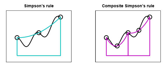
Composite Newton-Cotes¶

Preform Newton-Cotes on a grid separately on each interval

Equally spaced points
Newton-Cotes on each sub-interval

Note that the points are placed exogenously

Gaussian quadrature¶

General formula

$$ \int_a^b f(x) dx = \sum_{i=1}^n \omega_i f(x_i) $$

$ x_i \in [a,b] $ quadrature nodes
$ \omega_i $ quadrature weights

Note that the points are placed endogenously

Quadrature accuracy¶

Suppose that $ \{\phi_k(x)\}_{k=1,2,\dots} $ is family of polynomials of degree $ k $ orthogonal with respect to the weighting function $ w(x) $

let $ q_k $ denote the leading coefficients so that $ \phi_k(x)=q_k x^k + \dots $
let $ x_i $, $ i=1,\dots,n $ be $ n $ roots of $ \phi_n(x) $
let $ \omega_i = - \frac{q_{n+1}/q_n}{\phi'_n(x_i)\phi_{n+1}(x_i)}>0 $

Then

$ a<x_1<x_2<\dots<x_n<b $
for $ f(x) \in C^{(2n)}[a,b] $, for some $ \xi\in[a,b] $

$$ \int_a^b w(x) f(x) dx = \sum_{i=1}^n \omega_i f(x_i) + \frac{f^{(2n)}(\xi)}{q_n^2(2n)!} $$

the right hand side is unique on $ n $ nodes
exact integral for all polynomial $ f(x) $ of degree $ 2n-1 $

Gauss-Chebyshev Quadrature¶

Domain $ [-1,1] $
Weighting function $ (1-x^2)^{(-1/2)} $

$$ \int_{-1}^1 \frac{f(x)dx}{\sqrt{1-x^2}} = \frac{\pi}{n}\sum_{i=1}^{n} f(x_i) + \frac{\pi}{2^{2n-1}}\frac{f^{(2n)}(\xi)}{(2n)!} $$

quadrature nodes $ x_i = \cos(\frac{2i-1}{2n}\pi) $

Example¶

Want to integrate $ f(x) $ on $ [a,b] $, no weighting function.

Change of variable $ y=2(x-a)/(b-a)-1 $
Multiply and divide by weighting function

$$ \int_a^b f(x)dx = \frac{b-a}{2}\int_{-1}^{1}f\big(\frac{(y+1)(b-a)}{2}+a\big)\frac{\sqrt{1-y^2}}{\sqrt{1-y^2}}dy $$$$ \int_a^b f(x)dx = \frac{\pi(b-a)}{2n}\sum_{i=1}^{n}f\big(\frac{(y_i+1)(b-a)}{2}+a\big)\sqrt{1-y_i^2} $$

where $ y_i $ are Gauss-Chebyshev nodes over $ [-1,1] $

Gauss-Legendre Quadrature¶

Domain $ [-1,1] $
Weighting function $ 1 $

$$ \int_{-1}^1 f(x)dx = \sum_{i=1}^{n} \omega_i f(x_i) + \frac{2^{2n+1}(n!)^4}{(2n+1)!(2n)!} \frac{f^{(2n)}(\xi)}{(2n)!} $$

Nodes and weights come from Legendre polynomials, values tabulated

Gauss-Hermite Quadrature¶

Domain $ [-\infty,\infty] $
Weighting function $ \exp(-x^2) $

$$ \int_{-\infty}^\infty f(x) \exp(-x^2)dx = \sum_{i=1}^{n} \omega_i f(x_i) + \frac{n!\sqrt{\pi}}{2^n}\frac{f^{(2n)}(\xi)}{(2n)!} $$

Nodes and weights come from Hermite polynomials, values tabulated
Good for computing expectation with Normal distribution

Gauss-Laguerre Quadrature¶

Domain $ [0,\infty] $
Weighting function $ \exp(-x) $

$$ \int_{0}^\infty f(x) \exp(-x)dx = \sum_{i=1}^{n} \omega_i f(x_i) + (n!)^2\frac{f^{(2n)}(\xi)}{(2n)!} $$

Nodes and weights come from Laguerre polynomials, values tabulated
Good for computing expectation exponential discounting

Multidimensional quadrature¶

Much more complication, simple methods are subject to curse of dimensionality

Generic product rule

$$ \int_{[a,b]^d}f(x)dx=\sum_{i_1=1}^n \dots\sum_{i_d=1}^n \omega_{i_1}^1\dots\omega_{i_1}^d f(x_{i_1}^1,\dots,x^d_{i_d}) $$

Product Gaussian quadrature based on product orthogonal polynomials
Sparse methods
Monte Carlo integration!

Monte Carlo integration¶

Stochastic algorithm for computing integrals
Main idea: approximate the expectation of a function with an average computed from a sample of random draws
(convergence in the number of draws is due to the law of large numbers)
Then convert the integral in expectation to the integral of interest

Expectation of a function of random variable¶

let continuous random variable $ \tilde{X} $ be distributed with pdf $ p(x) $ over domain $ \Omega $
we are interested in the expectation of the function $ f(\tilde{X}) $ which is in turn a random variable itself

$$ E\big(f(\tilde{X})\big) = \int_{\Omega} f(x) \,dF(x) = \int_{\Omega} f(x) p(x) \,dx $$

variance of $ f(\tilde{X}) $ is

$$ \operatorname{Var} \big(f(\tilde{X})\big) = E\Big(f(\tilde{X})- E\big(f(\tilde{X})\big)\Big)^2 = E\big(f(\tilde{X})\big)^2 - \Big(E\big(f(\tilde{X})\big)\Big)^2 $$

From expectation to integration¶

imagine we want to compute the integral denoted $ I_f $ of function $ f(x) $ over some set $ \Omega $

$$ I_f =\int_{\Omega} f(x)\,dx $$

Step 1: represent the integral as an expectation of a function of some random variable $ \tilde{X} $ defined over domain $ \Omega $

$$ I_f =\int_{\Omega} f(x)\,dx = \int_{\Omega} \frac{f(x)}{p(x)} p(x) \,dx =E \left[ \frac{f(\tilde{X})}{p(\tilde{X})} \right] $$

From expectation to integration¶

Step 2: compute the expectation using $ N $ independent draws $ x_i $ of $ \tilde{X} $ — from the distribution with pdf $ p(x) $

$$ I_f =\int_{\Omega} f(x)\,dx = E \left[ \frac{f(\tilde{X})}{p(\tilde{X})} \right] \approx \frac{1}{N} \sum_{i=1}^{N} \frac{f(x_i)}{p(x_i)} \underset{N \rightarrow \infty}{\rightarrow} E \left[ \frac{f(\tilde{X})}{p(\tilde{X})} \right] $$

convergence due to the law of large numbers

Special simple case (naive Monte Carlo integration)¶

not to have to deal with pdf $ p(x) $ we can use uniform distribution
then pdf $ p(x) $ is independent of $ x $ and can be treated as a constant

$$ p(x) = \left( \int_{\Omega} dx \right) ^{-1} = \frac{1}{V} $$

$ V $ is a measure of the set $ \Omega $: length in one dimension, volume in two dimensions, etc.

$$ I_f =\int_{\Omega} f(x)\,dx = E \left[ Vf(\tilde{X}) \right] \approx \frac{V}{N} \sum_{i=1}^{N} f(x_i) $$

Special even simpler case with unit hypercube¶

let $ \Omega \subset \mathbb{R}^n $ be a unit hypercube denoted $ H_n $ in $ n $-dimensional space
then $ V = 1 $
integral is the same as simple average of the function computed on a random set of points uniformly distributed over the hypercube

$$ I_f =\int_{H_n} f(x)\,dx \approx \frac{1}{N} \sum_{i=1}^{N} f(x_i) $$

One dimensional example¶

let $ \Omega $ be an interval $ [a,b] \subset \mathbb{R} $ in one dimensional space
then $ V = b-a $

$$ I_f =\int_{a}^{b} f(x)\,dx \approx \frac{b-a}{N} \sum_{i=1}^{N} f(x_i) $$

One dimensional example visual¶

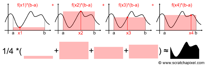
General Monte Carlo integration algorithm¶

sample $ N $ points $ x_1,\cdots,x_N $ from distribution $ p(x) $ of $ \tilde{X} $ on $ \Omega $
approximate the expectation $ E \left[ \frac{f(\tilde{X})}{p(\tilde{X})} \right] $ by the sample average

$$ I_f = \int_{\Omega} f(x)\,dx \approx \frac{1}{N} \sum_{i=1}^{N} \frac{f(x_i)}{p(x_i)} = Q_f(N) $$

General Monte Carlo integration algorithm (simple naive approach)¶

sample $ N $ points $ x_1,\cdots,x_N $ uniformly on $ \Omega $
approximate the expectation $ E \left[ V f(\tilde{X})\right] $ by the sample average

$$ I_f = \int_{\Omega} f(x)\,dx \approx \frac{V}{N} \sum_{i=1}^{N} f(x_i), \; V =\int_{\Omega} \,dx $$

In [1]:

import numpy as np
import matplotlib.pyplot as plt
%matplotlib inline
plt.rcParams['figure.figsize'] = [12, 8]

def mc_int_cube(f,ndims=1,N=1000):
    '''Computes the integral of function f on a hypercube of dimension ndims
       using Monte Carlo integration with N uniformly distributed points
       Assume function f uses axis=0 for inputs, and can be vectorized in other axis
       Return: value and standard error
    '''
    # generate uniform numbers on the hypercube
    x = np.random.random(ndims*N).reshape(ndims,N)  # uniform random numbers in a matrix
    y = f(x)                   # function value
    Q = y.mean()               # sample average
    seQ = y.std()/np.sqrt(N)   # standard error of sample average
    return Q,seQ

In [2]:

# pi example from video 33 as two-dim integral
# Approximate pi using 2-d Monte Carlo integration

N=1000 # Number of Monte carlo Samples
g = lambda x: (x[0,:]**2 + x[1,:]**2)<1  # indicator function to inegrate

q,se = mc_int_cube(g,ndims=2,N=N)
pi_hat = 4*q
se_pi_hat = 4*se

print('Number of Monte Carlo samples   : ', N);
print('Estimate (pi_hat)               : ', pi_hat.round(10));
print('Standard error (pi_hat)         : ', se_pi_hat.round(10));
print('Approximation error (pi_hat-pi) : ', (pi_hat-np.pi).round(10))

Number of Monte Carlo samples   :  1000
Estimate (pi_hat)               :  3.088
Standard error (pi_hat)         :  0.0530684087
Approximation error (pi_hat-pi) :  -0.0535926536

Properties of Monte Carlo integral¶

Consistency: Law of large numbers ensures that the sample average converge to the mean

$$ \lim _{{N\to \infty }}Q_f(N) =\lim _{{N\to \infty }}{\frac{1}{N}}\sum _{{i=1}}^{N}\frac{f(x_i)}{p(x_i)} =E\left[\frac{f(\tilde{x})}{p(\tilde{x})}\right] = \int_{\Omega} f(x)\,dx = I_f $$

Assymptotic Normality: By the central limit theorem we have

$$ \sqrt{N}\left(Q_f(N)-I_f \right)\ \xrightarrow {d} \ N\left(0,\sigma ^{2}\right), \; \sigma^2= \operatorname{Var}\left[\frac{f(\tilde{x})}{p(\tilde{x})}\right] $$

The standard error of $ Q_f(N) $ is then given by $ \sigma_{Q_f(N)}=\sigma \big/ \sqrt{N} $

Standard error of Monte Carlo integral¶

Given our estimate $ Q_f(N) $ of $ I_f $, we can obtain an unbiased estimate of $ \sigma^2= \operatorname{Var}\left[\frac{f(\tilde{x})}{p(\tilde{x})}\right] $

$$ {\hat{\sigma}}^2_N=\frac{1}{N-1}\sum _{i=1}^N \left(\frac{f(x_i)}{p(x_i)}-Q_f(N)\right)^2 $$

and the estimate of the standard error of $ Q_f(N) $

$$ {\hat{\sigma}}_{Q_f(N)}={\hat{\sigma}}_N \big/ \sqrt{N} $$

Convergence of Monte Carlo integrals¶

The standard error of $ Q_f(N) $:

is given by $ \sigma_{Q_f(N)}=\sigma \big/ \sqrt{N} $
can be estimated by $ {\hat{\sigma}}_{Q_f(N)}={\hat{\sigma}}_N \big/ \sqrt{N} $

Decreases with the standard parametric rate $ \sqrt{N} $

doubling of precision requires 4 time as many random points
but does not depend on the dimensionality of the integral, $ \Omega $ can be high dimensional

In [3]:

# distribution of Monte Carlo integral

N=1000; # number of Monte Carlo samples used to simulate the integral
S=1000; # number of runs to generate the distribution of estimates

qs = np.empty(S,dtype=float)
ses = np.empty(S,dtype=float)

for i in range(S):
    q,se = mc_int_cube(g,ndims=2,N=N)
    qs[i] = 4*q
    ses[i] = 4*se

plt.hist(qs,bins=50,range=(np.pi-.2, np.pi+.2))
plt.title('Distribution of %d Monte Carlo approximations of pi'%S)

print('True value (pi)                  :', np.round(np.pi,10))
print('Average estimate across all runs :', qs.mean().round(10))
print('Mean bias                        :', np.mean(qs-np.pi).round(10))
print('Average std err across all runs  :', ses.mean().round(10))
print('Std dev of bias                  :', np.std(qs-np.pi).round(10))

True value (pi)                  : 3.1415926536
Average estimate across all runs : 3.13976
Mean bias                        : -0.0018326536
Average std err across all runs  : 0.0519299844
Std dev of bias                  : 0.0533409261

Further learning resources¶

SciPy docs https://docs.scipy.org/doc/scipy/reference/tutorial/integrate.html
https://en.wikipedia.org/wiki/Gaussian_quadrature
Monte Carlo integration https://www.scratchapixel.com/lessons/mathematics-physics-for-computer-graphics/monte-carlo-methods-in-practice/monte-carlo-integration
Useful library for Monte Carlo methods https://chaospy.readthedocs.io/en/master/index.html