
O que é o IPython?

IPython é um ambiente para computação interativa e exploratória.
- Shell iterativo poderosos(Console, QtBased, WebBased)
- Arquitetura desacoplada com um Kernel que permite conexão com múltiplos clientes
- Arquitetura que permite programação paralela interativa
- Multi-linguagem de programção(Python, Ruby, R, Julia e Haskell)
- Opensource
IPython Notebook
IPython Notebook é um cliente do IPython com opções de interface rica acessível no navegor.
ipython notebook
Ao executar o comando um servidor do IPython Notebook será ativado e abrirá o dashboard.
O dashboard

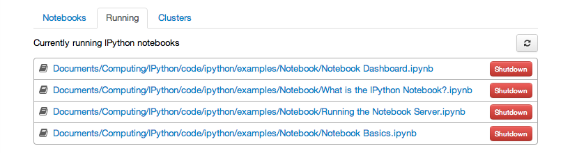
Running
A aba running mostra todos os notebooks que estão em execução
O notebook
Toolbar

Cells
Um notebook é composto por um conjunto de células que possuem dois modos: edição e comando
Modo de edição

Atalhos

Modo de comando

Atalhos

E o Python?
Cada célula do notebook pode ser uma execução de código Python
print "Hello, Pylestras!"
Tem dúvida sobre o código?
?
import collections
collections.namedtuple?
Além das docstrings você pode ver o código.
collections.Counter??
Lembra vagamente de uma função ou módulo Python?
*int*?
a = 1 + 2
print a
a
Você pode recuperar os Ins e Outs do histórico.
print In
print Out
Magic!

São um conjunto de funções para auxiliar em diversas tarefas. Os magics commands são prefixados por %
%magic
Magic podem ser de linha ou de Cell
%timeit range(100)
%%timeit
s = 0
for i in range(10):
    s += i ** 2
%%bash
echo "Meu path:"
pwd
[troll_mode] Ou você ainda pode extragar a brincadeira
%%ruby
6.times { puts 'Não faça isso em casa.' }
[/troll_mode]
%%javascript
alert("Hello, Pylestras");
%lsmagic
Acessando comandos do OS
!ls
files = !ls
for f in files:
    if f.endswith('.ipynb'):
        print f
python_variable = 42
!echo $python_variable
!echo {"{0:#b}".format(python_variable)}
Informações de conexão com o Kernel do IPython
%connect_info
%qtconsole
Plotando gráficos
%matplotlib inline
"""
Demo of the fill function with a few features.

In addition to the basic fill plot, this demo shows a few optional features:

    * Multiple curves with a single command.
    * Setting the fill color.
    * Setting the opacity (alpha value).
"""
import numpy as np
import matplotlib.pyplot as plt

x = np.linspace(0, 2 * np.pi, 100)
y1 = np.sin(x)
y2 = np.sin(3 * x)
plt.fill(x, y1, 'b', x, y2, 'r', alpha=0.3)
fig = plt.gcf()
%qtconsole
Suport a Markdown
Você pode usar markdown ou HTML.
| This | is   |
|------|------|
|   a  | table|
A tabela será renderizada em HTML
| This | is |
|---|---|
| a | table |
Suporte a LaTeX
O IPython Notebook usa MathJax para rederizar expressões matemáticas usando LaTeX. Pode ser em linha: $e^{i\pi} + 1 = 0$ ou em bloco:
$$e^x=\sum_{i=0}^\infty \frac{1}{i!}x^i$$Elementos ricos com Python
Imagens
from IPython.display import Image
Image(url='http://python.org/images/python-logo.gif')
Image('http://ipython.org/_static/IPy_header.png')
Vídeos do Youtube
from IPython.display import YouTubeVideo
YouTubeVideo('kkwiQmGWK4c')
Audio
from IPython.display import Audio
import numpy as np
import matplotlib.pyplot as plt
max_time = 3
f1 = 220.0
f2 = 224.0
rate = 44100.0
L = 3
times = np.linspace(0,L,rate*L)
signal = np.sin(2*np.pi*f1*times) + np.sin(2*np.pi*f2*times)

Audio(data=signal, rate=rate)
audio_plt = plt.plot(times, signal)
Usando sympy para símbolos matemáticos
from sympy import *
init_printing()
x = Symbol('x')
(pi + x)**2
(x+1)*(x+2)*(x+3)
expand((x+1)*(x+2)*(x+3))
Widgets interativos
from IPython.html.widgets import interact, interactive, fixed
def f(x):
    print x
interact(f, x=10);
interact(f, x=True);
interact(f, x='Hi there!');
@interact(x=True, y=1.0)
def g(x, y):
    print(x, y)
Exemplo completo com o scikit-image
import skimage
from skimage import data, filter, io

from IPython.display import display
i = data.coffee()
lims = (0.0,1.0,0.01)

def edit_image(image, sigma=0.1, r=1.0, g=1.0, b=1.0):
    new_image = filter.gaussian_filter(image, sigma=sigma, multichannel=True)
    new_image[:,:,0] = r*new_image[:,:,0]
    new_image[:,:,1] = g*new_image[:,:,1]
    new_image[:,:,2] = b*new_image[:,:,2]
    new_image = io.Image(new_image)
    display(new_image)
    return new_image

w = interactive(edit_image, image=fixed(i), sigma=(0.0,10.0,0.1), r=lims, g=lims, b=lims)
display(w)
Integração com Pandas para manipulação de dados
import pandas as pd
ts = pd.Series(np.random.randn(10), index=pd.date_range('1/1/2014', periods=10))
df = pd.DataFrame(np.random.randn(10, 4), index=ts.index,
                  columns=['A', 'B', 'C', 'D'])

df = df.cumsum()
df
plt.figure()
df.plot()
plt.legend(loc='best')
Disponiblizando seus notebooks no nbviewer
from IPython.display import IFrame
IFrame('http://nbviewer.ipython.org/', 800, 600)
Referência
- Esse tutorial é completamente baseado no vídeo do Fernando Perez
- http://www.scipy.org/
- http://ipython.org