%pylab inline
import sklearn
Populating the interactive namespace from numpy and matplotlib
# Visualizes how a classifier would classify each point in a grid
# http://scikit-learn.org/stable/auto_examples/neighbors/plot_classification.html

from matplotlib.colors import ListedColormap
def decision_boundary(clf, X, Y):
    h = .02  # step size in the mesh

    # Create color maps
    cmap_light = ListedColormap(['#FFAAAA', '#AAFFAA', '#AAAAFF'])
    cmap_bold = ListedColormap(['#FF0000', '#00FF00', '#0000FF'])

    # Plot the decision boundary. For that, we will assign a color to each
    # point in the mesh [x_min, m_max] x[y_min, y_max].
    x_min, x_max = X[:, 0].min() - 1, X[:, 0].max() + 1
    y_min, y_max = X[:, 1].min() - 1, X[:, 1].max() + 1
    xx, yy = np.meshgrid(np.arange(x_min, x_max, h),
                         np.arange(y_min, y_max, h))
    Z = clf.predict(np.c_[xx.ravel(), yy.ravel()])

    # Put the result into a color plot
    Z = Z.reshape(xx.shape)
    plt.figure()
    plt.pcolormesh(xx, yy, Z, cmap=cmap_light)

    # Plot also the training points
    plt.scatter(X[:, 0], X[:, 1], c=Y, cmap=cmap_bold)
    plt.xlim(xx.min(), xx.max())
    plt.ylim(yy.min(), yy.max())

    plt.show()
def plot_test_train(clf, Xtrain, Ytrain, Xtest):
    plt.prism()  # this sets a nice color map
    plt.scatter(Xtest[:, 0], Xtest[:, 1], c=clf.predict(Xtest), marker='^')
    plt.scatter(Xtrain[:, 0], Xtrain[:, 1], c=Ytrain)
Installing sklearn
sklearn requires depends on numpy and scipy.
pip install numpy scipy scikit-learn
It's also helpful to have matplotlib
pip install matplotlib
Installation on a Mac can be tricky. Take a look at here for more details.
Example data: MNIST
We'll use the MNIST digit dataset for classification
from sklearn.datasets import load_digits
digits = load_digits()
print("images shape: %s" % str(digits.images.shape))
print("targets shape: %s" % str(digits.target.shape))
digit_X = digits.images.reshape(-1, 64)  # Reshape 8x8 images to length 64 vectors
digit_Y = digits.target # Get labels
images shape: (1797, 8, 8)
targets shape: (1797,)
plt.matshow(digits.images[0], cmap=plt.cm.Greys);

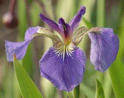
Example data: Iris
We'll also use the iris dataset, which consists of data from three types of irises (Setosa, Versicolour, and Virginica). Features are measurements of
- Sepal Length
- Sepal Width
- Petal Length
- Petal Width.
from sklearn.datasets import load_iris
iris = load_iris()
print iris.data.shape
(150, 4)
Example data: Iris
IX  = iris.data # Get features
IY = iris.target # Get labels
print("X shape: {}".format(IX.shape))
print("Example features:\n {}".format(IX[:5]))
print("Labels:\n {}".format(IY[:70]))
X shape: (150, 4)
Example features:
 [[ 5.1  3.5  1.4  0.2]
 [ 4.9  3.   1.4  0.2]
 [ 4.7  3.2  1.3  0.2]
 [ 4.6  3.1  1.5  0.2]
 [ 5.   3.6  1.4  0.2]]
Labels:
 [0 0 0 0 0 0 0 0 0 0 0 0 0 0 0 0 0 0 0 0 0 0 0 0 0 0 0 0 0 0 0 0 0 0 0 0 0
 0 0 0 0 0 0 0 0 0 0 0 0 0 1 1 1 1 1 1 1 1 1 1 1 1 1 1 1 1 1 1 1 1]
Getting started: Classification with K-Nearest Neighbors
First we generate sample data:
from sklearn.datasets import make_blobs
BX, BY = make_blobs(cluster_std=1.6, random_state=9)
plt.scatter(BX[:, 0], BX[:, 1], c=BY);plt.show()

Now training a simple KNN classifier
from sklearn.neighbors import KNeighborsClassifier

knn = KNeighborsClassifier(n_neighbors=1)

knn.fit(BX, BY)
decision_boundary(knn, BX, BY)

Let's try a larger k
knn = KNeighborsClassifier(n_neighbors=10)

knn.fit(BX, BY)
decision_boundary(knn, BX, BY)

Applying to Iris
Applying the same technique to Iris is simple:
X, Y = sklearn.utils.shuffle(IX, IY)

for k in [1,3,5]:
    knn = KNeighborsClassifier(n_neighbors=k)
    for n in [10, 50, 100]:
        knn.fit(X[:n], Y[:n])
        print("{} {}: {}".format(k, n, knn.score(X[n:], Y[n:])))
    print
1 10: 0.85
1 50: 0.93
1 100: 0.96

3 10: 0.8
3 50: 0.92
3 100: 0.96

5 10: 0.664285714286
5 50: 0.95
5 100: 0.98
Avoiding overfitting
- Overfitting: fitting a model to details of your training data that don't generalize.
- Testing on a held out test set gives an estimate of generalization error
- Ideally, one has a "gold standard" test set (separate from validation set) that is never used for fitting parameters
from sklearn.cross_validation import train_test_split

# Test on 1/3 of data
X_train, X_test, Y_train, Y_test = train_test_split(IX, IY, test_size=0.33)

knn = KNeighborsClassifier(n_neighbors=3)
knn.fit(X_train, Y_train)
knn.score(X_test, Y_test)
0.95999999999999996
KFold Cross validation
This method splits the data into folds so that every example is held out in the test set exactly once.
from sklearn.cross_validation import KFold
from sklearn.metrics import accuracy_score

def score(clf, X, Y, folds=2, verbose=False, metric=accuracy_score):
    predictions = np.zeros(len(Y))
    for i, (train, test) in enumerate(KFold(len(X), n_folds=folds, shuffle=True)):
        clf.fit(X[train], Y[train])
        predictions[test] = clf.predict(X[test])
        if verbose:
            print("Fold {}: {}".format(i + 1, accuracy_score(Y[test], predictions[test])))
    if metric:
        return metric(Y, predictions)
    return Y, predictions
KFold Cross validation
We can use such a method to test out different parameter settings
for k in range(1, 10, 2):
    acc = score(KNeighborsClassifier(n_neighbors=k), IX, IY, folds=30)
    print("{}: {}".format(k, acc))
1: 0.96
3: 0.96
5: 0.966666666667
7: 0.966666666667
9: 0.966666666667
On the dataset of 150 examples, this does 5 splits of 120 training/30 testing examples
Random Forests
Random forests are an ensemble technique: they combine many decision trees
Decision trees classify an instance by repeatedly branching on features until they reach a labelled node
from sklearn import tree

dt = tree.DecisionTreeClassifier()
dt.fit(BX, BY)
decision_boundary(dt, BX, BY)

Random Forests
Random forests train many decision trees on subsets of features and data and combine the individual predictions
from sklearn.ensemble import RandomForestClassifier

df = RandomForestClassifier(n_estimators=10)
df.fit(BX, BY)
decision_boundary(df, BX, BY)

Support Vector Machines
SVMs attempt to find a hyperplane that separates different classes. In 2d, this is just a line.
from sklearn import svm

clf = svm.SVC(kernel='linear')
clf.fit(BX, BY)
decision_boundary(clf, BX, BY)

Support Vector Machines
Things get trickier when your data isn't linearly separable. For example:
from sklearn.datasets import make_circles
CX, CY = make_circles(factor=0.5, noise=0.2, random_state=1)
clf = svm.SVC(kernel='linear')
clf.fit(CX, CY)
decision_boundary(clf, CX, CY)

SVM Kernels
SVMs get around this by projecting data into a space where it is linearly separable.
# Illustrate linearSVM on Circle dataset
clf = svm.SVC(kernel='rbf') # rbf is the default kernel type
clf.fit(CX, CY)
decision_boundary(clf, CX, CY)

SVM Kernels
The default rbf kernel is a safe bet in most cases
# Illustrate linearSVM on Circle dataset
clf = svm.SVC()
clf.fit(BX, BY)
decision_boundary(clf, BX, BY)

Multiclass classification
While SVMs are generally a safe default, they are not ideal for data with many classes.
If there are many classes, consider using alternative classifiers such as random forests.
Inspecting results: Metrics
Aggregate classification accuracy is a coarse measure of performance. sklearn provides many metrics to get a better sense of what's going on.
from sklearn import metrics
clf = svm.SVC()
y, pred = score(clf, IX, IY, metric=None)
print(metrics.classification_report(y, pred))
print(metrics.confusion_matrix(y, pred))
             precision    recall  f1-score   support

          0       1.00      1.00      1.00        50
          1       0.92      0.98      0.95        50
          2       0.98      0.92      0.95        50

avg / total       0.97      0.97      0.97       150

[[50  0  0]
 [ 0 49  1]
 [ 0  4 46]]
clf = svm.SVC()
y, pred = score(clf, digit_X, digit_Y, folds=10, metric=None)
print(metrics.classification_report(y, pred))
print(metrics.confusion_matrix(y, pred))
             precision    recall  f1-score   support

          0       1.00      0.54      0.71       178
          1       1.00      0.45      0.62       182
          2       1.00      0.46      0.63       177
          3       0.33      0.74      0.45       183
          4       1.00      0.52      0.68       181
          5       0.25      0.76      0.37       182
          6       1.00      0.66      0.79       181
          7       1.00      0.49      0.65       179
          8       1.00      0.16      0.27       174
          9       0.45      0.59      0.51       180

avg / total       0.80      0.54      0.57      1797

[[ 97   0   0  21   0  44   0   0   0  16]
 [  0  81   0  34   0  51   0   0   0  16]
 [  0   0  81  48   0  40   0   0   0   8]
 [  0   0   0 135   0  45   0   0   0   3]
 [  0   0   0  34  94  45   0   0   0   8]
 [  0   0   0  31   0 138   0   0   0  13]
 [  0   0   0  22   0  23 119   0   0  17]
 [  0   0   0  23   0  55   0  87   0  14]
 [  0   0   0  40   0  71   0   0  27  36]
 [  0   0   0  23   0  50   0   0   0 107]]
clf = svm.SVC(kernel='linear') #This is a case where a different kernel helps
y, pred = score(clf, digit_X, digit_Y, folds=10, metric=None)
print(metrics.classification_report(y, pred))
print(metrics.confusion_matrix(y, pred))
             precision    recall  f1-score   support

          0       1.00      0.99      1.00       178
          1       0.96      0.98      0.97       182
          2       0.99      1.00      1.00       177
          3       0.98      0.97      0.98       183
          4       0.98      0.99      0.99       181
          5       0.96      0.98      0.97       182
          6       1.00      0.98      0.99       181
          7       0.98      0.98      0.98       179
          8       0.95      0.94      0.94       174
          9       0.97      0.96      0.96       180

avg / total       0.98      0.98      0.98      1797

[[177   0   0   0   1   0   0   0   0   0]
 [  0 179   0   0   0   0   0   0   3   0]
 [  0   0 177   0   0   0   0   0   0   0]
 [  0   0   0 178   0   2   0   0   3   0]
 [  0   0   0   0 180   0   0   1   0   0]
 [  0   0   0   1   0 178   0   0   0   3]
 [  0   1   0   0   1   0 178   0   1   0]
 [  0   0   0   0   1   1   0 176   0   1]
 [  0   6   1   0   1   1   0   1 163   1]
 [  0   0   0   2   0   3   0   1   2 172]]
Linear Regression
Regression attempts to predict continuous values rather than discrete labels.
sklearn has many different many different types of regression, but they all follow the fit/predict paradigm.
This example uses a dataset of house prices:
from sklearn.datasets import load_boston
data = load_boston()
HX = data['data']
HY = data['target']
print data.DESCR[:1200]
Boston House Prices dataset

Notes
------
Data Set Characteristics:

    :Number of Instances: 506

    :Number of Attributes: 13 numeric/categorical predictive

    :Median Value (attribute 14) is usually the target

    :Attribute Information (in order):
        - CRIM     per capita crime rate by town
        - ZN       proportion of residential land zoned for lots over 25,000 sq.ft.
        - INDUS    proportion of non-retail business acres per town
        - CHAS     Charles River dummy variable (= 1 if tract bounds river; 0 otherwise)
        - NOX      nitric oxides concentration (parts per 10 million)
        - RM       average number of rooms per dwelling
        - AGE      proportion of owner-occupied units built prior to 1940
        - DIS      weighted distances to five Boston employment centres
        - RAD      index of accessibility to radial highways
        - TAX      full-value property-tax rate per $10,000
        - PTRATIO  pupil-teacher ratio by town
        - B        1000(Bk - 0.63)^2 where Bk is the proportion of blacks by town
        - LSTAT    % lower status of the population
        - MEDV     Median value of owner-occupied homes in $1000's
Linear Regression
Let's try vanilla linear regression:
from sklearn import linear_model as lm

y, pred = score(lm.LinearRegression(), HX, HY, folds=10, metric=None)
print(metrics.mean_squared_error(y, pred))
24.2456385287
To put this in context, take a look at the price distribution:
plt.hist(HY);plt.show()

# Example discovered cluster centers
from sklearn import cluster
km = cluster.KMeans(n_clusters=3)
Y_hat = km.fit(BX).labels_

plt.scatter(BX[:,0], BX[:,1], c=BY, alpha=0.4)
mu = km.cluster_centers_
plt.scatter(mu[:,0], mu[:,1], s=100, c=np.unique(Y_hat))
plt.show()


from sklearn.decomposition import RandomizedPCA
pca = RandomizedPCA(n_components=2)
proj = pca.fit_transform(digits.data)
plt.scatter(proj[:, 0], proj[:, 1], c=digits.target)
plt.colorbar();plt.show()

from sklearn.decomposition import RandomizedPCA
pca = RandomizedPCA(n_components=2)
proj = pca.fit_transform(IX)
plt.scatter(proj[:, 0], proj[:, 1], c=IY)
plt.colorbar();plt.show()

Dimensionality reduction: Manifold learning
Manifold learning is another approach to mapping data to a lower dimensional space.
There are many different types of manifold learning in sklearn. In practice, PCA is a safe bet.
from sklearn.manifold import Isomap
iso = Isomap(n_neighbors=5, n_components=2)
proj = iso.fit_transform(digits.data)
plt.scatter(proj[:, 0], proj[:, 1], c=digits.target)
plt.colorbar();plt.show()

#from sklearn.manifold import MDS
#mds = MDS()
#proj = mds.fit_transform(digit_X)
#plt.scatter(proj[:, 0], proj[:, 1], c=digit_Y)
#plt.colorbar();plt.show()
Choosing parameters: Grid Search
Grid search is a method for systematically testing model performance with various parameter settings
from sklearn.grid_search import GridSearchCV

param_grid = [
    {'C': [1, 10], 'kernel': ['linear']},
    {'C': [1, 10], 'gamma': [0.001, 0.0001], 'kernel': ['rbf']},
 ]

gs = GridSearchCV(svm.SVC(), param_grid)
gs.fit(digit_X, digit_Y) # Let's try it on MNIST
print(gs.best_params_)
print(gs.grid_scores_)

gs.fit(IX, IY) # Different settings work better for the iris dataset
print(gs.best_params_)
print(gs.grid_scores_)
{'kernel': 'rbf', 'C': 1, 'gamma': 0.001}
[mean: 0.98164, std: 0.00136, params: {'kernel': 'linear', 'C': 1}, mean: 0.98164, std: 0.00136, params: {'kernel': 'linear', 'C': 10}, mean: 0.99110, std: 0.00284, params: {'kernel': 'rbf', 'C': 1, 'gamma': 0.001}, mean: 0.97051, std: 0.00799, params: {'kernel': 'rbf', 'C': 1, 'gamma': 0.0001}, mean: 0.99054, std: 0.00208, params: {'kernel': 'rbf', 'C': 10, 'gamma': 0.001}, mean: 0.98497, std: 0.00491, params: {'kernel': 'rbf', 'C': 10, 'gamma': 0.0001}]
{'kernel': 'linear', 'C': 1}
[mean: 0.98000, std: 0.01633, params: {'kernel': 'linear', 'C': 1}, mean: 0.96667, std: 0.00943, params: {'kernel': 'linear', 'C': 10}, mean: 0.52000, std: 0.14514, params: {'kernel': 'rbf', 'C': 1, 'gamma': 0.001}, mean: 0.32000, std: 0.00000, params: {'kernel': 'rbf', 'C': 1, 'gamma': 0.0001}, mean: 0.90000, std: 0.01633, params: {'kernel': 'rbf', 'C': 10, 'gamma': 0.001}, mean: 0.52000, std: 0.14514, params: {'kernel': 'rbf', 'C': 10, 'gamma': 0.0001}]
Combining models: Pipelines
We can combine many models together in a pipeline. The final step in the pipeline is a classifier, and all other steps are feature transforms
A simple pipeline could use PCA to project the data into 3 dimensions before classifying with an SVM
from sklearn.pipeline import Pipeline

pca = RandomizedPCA(n_components=16)
clf = svm.SVC(kernel='linear')

pipeline = Pipeline(steps=[('PCA', pca), ('SVM', clf)])

# fit/predict work in the same way as other classifiers
# pipeline.fit(X[train], Y[train])
# pipeline.predict(X[test], Y[test])

score(pipeline, digit_X, digit_Y, folds=10)
0.96215915414579856
Putting it all together: Facial recognition
Putting it all together: Image classification
Putting it all together: Working with Text
Attributions
This presentation has been pieced together from my own knowledge and tutorials such as the Scipy2013 sklearn tutorial mentioned above (particularly for some visualizations and the eigenfaces example). Other sources include Andreas Mueller's excellent sklearn presentation and the many tutorials available in the sklearn documentation.