[PUBLIC LECTURE AT DEEPHACK.RL]
Cross-platform multi-objective optimisation via Collective Knowledge
from IPython.display import Image
from IPython.core.display import HTML
Image(url="http://dividiti.com/dvdt/a_eq_dvdt_1000.png")

Motivation: Autonomous Driving
No, that's not quite what we mean!
Image(url="http://taxistartup.com/wp-content/uploads/2015/03/UK-Self-Driving-Cars.jpg")

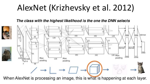
Convolutional Neutral Networks are the state-of-the-art
Image(url="http://image.slidesharecdn.com/pydatatalk-150729202131-lva1-app6892/95/deep-learning-with-python-pydata-seattle-2015-35-638.jpg?cb=1438315555")
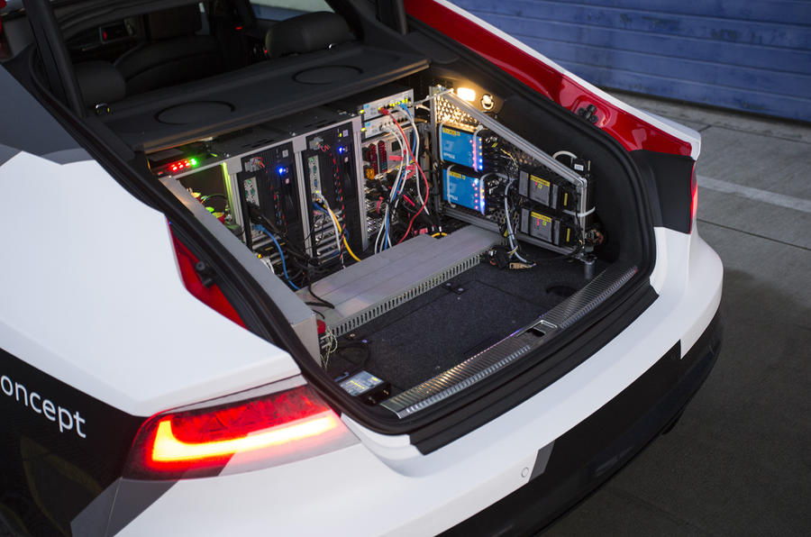
Today proof-of-concepts: ~10,000 W, ~$10,000, and, look, no space for luggage!
Image(url="http://images.cdn.autocar.co.uk/sites/autocar.co.uk/files/styles/gallery_slide/public/audi-rs7-driverless-005.jpg?itok=A-GlUErw")
Need 3-4 orders of magnitude improvement in terms of performance, power, cost, space!
Image(url="https://1.bp.blogspot.com/-aQw-r1FZcQk/VyINpA8ntxI/AAAAAAAAPF4/o34l1MvKJVQTuLD1qsv5Ink-04Dra0PDgCLcB/s1600/Movidius%2BFathom-1.JPG")

Table of Contents
- Overview
- See the code [for developers]
- Get the data [for developers]
- See the tables
- Accuracy
- All data
- All execution time data
- Mean execution time per batch
- Mean execution time per image
- Best mean execution time per image
- See the graphs - grouped by models
- Accuracy
- All libs
- GPU libs
- CUDA-level performance libs
- cuBLAS libs
- cuDNN libs
- See the graphs - grouped by libs
- All models
- All models, GPU libs
- Models with AlexNet-level accuracy
- Models with AlexNet-level accuracy, CPU lib
- Models with AlexNet-level accuracy, CUDA-level perfomance libs
- Models with AlexNet-level accuracy, fp16 libs
- GoogleNet, fp16 libs
- See the graphs - per layer execution time profiling
- See the graphs - the ideal adaptive solution
- Using all libs for adaptation
- Using CUDA-level performance libs for adaptation
- Using cuDNN and cuBLAS for adaptation
- Using cuDNN and libDNN for adaptation
- See the memory consumption graph
- Balance memory consumption and execution time per image
- Compare AlexNet and SqueezeNet 1.1
- Compare memory consumption
- Compare execution time
- Conclusion
- What are the improvements brought on by each approach?
- How does TX1 compare to Myriad2?
- Collective Knowledge on Deep Learning
Overview
This Jupyter Notebook compares the performance (execution time, memory consumption):
- on dividiti's Jetson TX1 board (official page, Phoronix review):
- CPU:
- ARM® Cortex®-A57 architecture ("big");
- 4 cores;
- Max clock 1743 MHz;
- GPU:
- Maxwell™ architecture;
- 256 CUDA cores;
- Max clock 998 MHz;
- RAM:
- LPDDR4;
- 4 GB (shared between the CPU and the GPU);
- Max bandwidth 25.6 GB/s;
- Linux for Tegra 24.2.1;
- JetPack 2.3.1;
- CUDA Toolkit 8.0.33.
- CPU:
$ uname -a
Linux tegra-ubuntu 3.10.96-tegra #1 SMP PREEMPT Wed Nov 9 19:42:57 PST 2016 aarch64 aarch64 aarch64 GNU/Linux
$ cat /etc/lsb-release
DISTRIB_ID=Ubuntu
DISTRIB_RELEASE=16.04
DISTRIB_CODENAME=xenial
DISTRIB_DESCRIPTION="Ubuntu 16.04.1 LTS"
using 8 Caffe libraries:
- [
tag] Branch (revision hash, date): math libraries. - [
cpu] Master (24d2f67, 28/Nov/2016): with OpenBLAS 0.2.19; - [
cuda] Master (24d2f67, 28/Nov/2016): with cuBLAS (part of CUDA Toolkit 8.0.33); - [
cudnn] Master 24d2f67, 28/Nov/2016): with cuDNN 5.1; - [
libdnn-cuda] OpenCL (b735c2d, 23/Nov/2016): with libDNN and cuBLAS (NB: not yet tuned for TX1; uses optimal parameters for GTX 1080); - [
nvidia-cuda] NVIDIA v0.15 (1024d34, 17/Nov/2016): with cuBLAS (part of CUDA Toolkit 8.0.33); - [
nvidia-cudnn] NVIDIA v0.15 (1024d34, 17/Nov/2016): with cuDNN 5.1; - [
nvidia-fp16-cuda] NVIDIA experimental/fp16 (fca1cf4, 11/Jul/2016): with cuBLAS (part of CUDA Toolkit 8.0.33); - [
nvidia-fp16-cudnn] NVIDIA experimental/fp16 (fca1cf4, 11/Jul/2016): with cuDNN 5.1;
- [
using 4 CNN models:
with the batch size varying from 2 to 16 with step 2.
Configure the execution time metric to use
fw = [ 'forward' ]
fwbw = [ 'forward', 'backward' ]
# Set to fw for inference; to fwbw for training.
direction = fw
direction
['forward']
if direction==fw:
    time_ms = 'time_fw_ms'
else: # direction==fwbw
    time_ms = 'time_fwbw_ms'
time_ms
'time_fw_ms'
def images_per_second(time_in_milliseconds):
    return 1000.0 / time_in_milliseconds
Data wrangling code
NB: Please ignore this section if you are not interested in re-running or modifying this notebook.
Includes
Standard
import os
import sys
import json
import re
Scientific
If some of the scientific packages are missing, please install them using:
# pip install jupyter pandas numpy matplotlib
import IPython as ip
import pandas as pd
import numpy as np
import matplotlib as mp
print ('IPython version: %s' % ip.__version__)
print ('Pandas version: %s' % pd.__version__)
print ('NumPy version: %s' % np.__version__)
print ('Matplotlib version: %s' % mp.__version__)
IPython version: 5.1.0
Pandas version: 0.19.0
NumPy version: 1.11.2
Matplotlib version: 1.5.3
import matplotlib.pyplot as plt
from matplotlib import cm
%matplotlib inline
Collective Knowledge
If CK is not installed, please install it using:
# pip install ck
import ck.kernel as ck
print ('CK version: %s' % ck.__version__)
CK version: 1.8.6.1
Pretty print libs and models
pretty_print_libs = {
    'cpu':              '[CPU] OpenBLAS',
    'libdnn-cuda':      '[GPU] libDNN-fp32',
    'nvidia-cuda':      '[GPU] cuBLAS-fp32',
    'nvidia-fp16-cuda': '[GPU] cuBLAS-fp16',
    'nvidia-cudnn':     '[GPU] cuDNN-fp32',
    'nvidia-fp16-cudnn':'[GPU] cuDNN-fp16'
}

pretty_print_models = {
    'bvlc-alexnet':'AlexNet',
    'bvlc-googlenet':'GoogleNet',
    'deepscale-squeezenet-1.0':'SqueezeNet 1.0',
    'deepscale-squeezenet-1.1':'SqueezeNet 1.1'
}

speedup_sort_models = [
    '[CPU] OpenBLAS',
    '[GPU] libDNN-fp32',
    '[GPU] cuBLAS-fp32',
    '[GPU] cuBLAS-fp16',
    '[GPU] cuDNN-fp32',
    '[GPU] cuDNN-fp16'
]
Access the experimental data
def get_experimental_results(repo_uoa, tags):
    module_uoa = 'experiment'
    r = ck.access({'action':'search', 'repo_uoa':repo_uoa, 'module_uoa':module_uoa, 'tags':tags})
    if r['return']>0:
        print ("Error: %s" % r['error'])
        exit(1)
    experiments = r['lst']

    dfs = []
    for experiment in experiments:
        data_uoa = experiment['data_uoa']
        r = ck.access({'action':'list_points', 'repo_uoa':repo_uoa, 'module_uoa':module_uoa, 'data_uoa':data_uoa})
        if r['return']>0:
            print ("Error: %s" % r['error'])
            exit(1)

        # Get (lib_tag, model_tag) from a list of tags that should be available in r['dict']['tags'].
        # Tags include 2 of the 3 irrelevant tags, a model tag and a lib tag.
        # NB: Since it's easier to list all model tags than all lib tags, the latter list is not expicitly specified.
        tags = r['dict']['tags']
        irrelevant_tags = [ 'explore-batch-size-libs-models','time_gpu','time_cpu','time_gpu_fp16' ]
        model_tags = [ 'bvlc-alexnet','bvlc-googlenet','deepscale-squeezenet-1.0','deepscale-squeezenet-1.1' ]
        lib_model_tags = [ tag for tag in tags if tag not in irrelevant_tags ]
        model_tags = [ tag for tag in lib_model_tags if tag in model_tags ]
        lib_tags = [ tag for tag in lib_model_tags if tag not in model_tags ]
        if len(lib_tags)==1 and len(model_tags)==1:
            (lib, model) = (lib_tags[0], model_tags[0])
        else:
            continue

        for point in r['points']:
            with open(os.path.join(r['path'], 'ckp-%s.0001.json' % point)) as point_file:
                point_data_raw = json.load(point_file)
                # Obtain column data.
                characteristics = [
                    {
                        'time (ms)'   : characteristics['run'].get(time_ms,+1e9), # "positive infinity"
                        'memory (MB)' : characteristics['run'].get('memory_mbytes',-1),
                        'success?'    : characteristics['run'].get('run_success','n/a'),
                        'per layer info' : characteristics['run'].get('per_layer_info',[])
                    }
                    for characteristics in point_data_raw['characteristics_list']
                ]
                # Deal with missing column data (resulting from failed runs).
                if len(characteristics)==1:
                    repetitions = point_data_raw['features'].get('statistical_repetitions',1)
                    characteristics = characteristics * repetitions
                # Construct a DataFrame.
                df = pd.DataFrame(characteristics)
                # Set columns and index names.
                df.columns.name = 'run characteristic'
                df.index.name = 'repetition'
                # Set indices.
                if lib=='tensorrt-1.0.0':
                    enable_fp16 = (point_data_raw['choices']['env']['CK_TENSORRT_ENABLE_FP16'] != 0)
                    df['lib'] = 'tensorrt-fp%d' % (16 if enable_fp16 else 32)
                else:
                    df['lib'] = lib
                df['model'] = model
                df['batch size'] = point_data_raw['choices']['env']['CK_CAFFE_BATCH_SIZE']
                df = df.set_index(['lib', 'model', 'batch size'], append=True)
                df = df.reorder_levels(('model', 'lib', 'batch size', 'repetition'))
                # Append to the list of similarly constructed DataFrames.
                dfs.append(df)
    # Concatenate all constructed DataFrames (i.e. stack on top of each other).
    result = pd.concat(dfs)
    return result.sortlevel(result.index.names)
Plot execution time per image or memory consumption
def plot(mean, std, title='Execution time per image (ms)', ymax=0, rot=0):
    ymax = mean.max().max() if ymax==0 else ymax
    mean.plot(yerr=std, ylim=[0,ymax*1.05], title=title,
        kind='bar', rot=rot, figsize=[16, 8], grid=True, legend=True, colormap=cm.autumn)
Plot maximum number of images per second
# ['cuda', 'cudnn'] are roughly equivalent to ['nvidia-cuda', 'nvidia-cudnn'], so can be dropped.
def plot_max_num_images_per_second(df_mean_time_per_image, libs_to_drop=['cuda', 'cudnn'], rot=0):
    min_time_per_image = df_mean_time_per_image.min(axis=1).unstack('lib')
    max_num_images_per_second = images_per_second(min_time_per_image) \
        .drop(libs_to_drop, axis=1) \
        .rename(columns=pretty_print_libs, index=pretty_print_models) \
        .reindex(columns=speedup_sort_models)
    ax = max_num_images_per_second \
            .plot(title='Images/s (with the best even batch size between 2 and 16)', kind='bar',
                  figsize=[16, 8], width=0.95, rot=rot, grid=True, legend=True, colormap=cm.autumn)
    for patch in ax.patches:
         ax.annotate(str(int(patch.get_height()+0.5)), (patch.get_x()*1.00, patch.get_height()*1.01))
Plot the speedup over a given baseline
# ['cuda', 'cudnn'] are roughly equivalent to ['nvidia-cuda', 'nvidia-cudnn'], so can be dropped.
def plot_speedup_over_baseline(df_mean_time_per_image, baseline='cpu', libs_to_drop=['cuda', 'cudnn'], rot=0):
    speedup_over_baseline = df_mean_time_per_image.min(axis=1).unstack('model').ix[baseline] / \
                            df_mean_time_per_image.min(axis=1).unstack('model')
    speedup_over_baseline = speedup_over_baseline.T \
        .drop(libs_to_drop, axis=1) \
        .rename(columns=pretty_print_libs, index=pretty_print_models) \
        .reindex(columns=speedup_sort_models)
    ax = speedup_over_baseline \
            .plot(title='Speedup over the given baseline (%s)' % pretty_print_libs[baseline], kind='bar',
                  figsize=[16, 8], width=0.95, rot=rot, grid=True, legend=True, colormap=cm.autumn)
    for patch in ax.patches:
        ax.annotate('{0:.2f}'.format(patch.get_height())[0:4], (patch.get_x()*1.00, patch.get_height()*1.01))
Plot execution time per image per layer
# This transformation is time consuming, hence only call it once for multiple plots.
def get_per_layer_info(df_all):
    df_per_layer_info = df_all['per layer info']
    row_dfs = []
    for (row_info, row_id) in zip(df_per_layer_info, range(len(df_per_layer_info))):
        # Skip constructing a DataFrame when no layer info is available.
        if not row_info: continue
        # Augment each layer info with the row index: (model, lib, batch size, repetition).
        for layer_info in row_info:
            layer_info.update({ k : v for k, v in zip(df_per_layer_info.index.names, df_per_layer_info.index[row_id]) })
        # Construct a DataFrame and move the row index to where it belongs.
        row_df = pd.DataFrame(data=row_info).set_index(df_per_layer_info.index.names)
        row_dfs.append(row_df)
    return pd.concat(row_dfs)
def plot_time_per_image_per_layer(df_per_layer_info, model, libs, batch_sizes,
                                  direction=['forward'], lower=0.0, upper=1.0, ymax=0, rot=90):
    df_time_per_batch = df_per_layer_info.loc[model, libs, batch_sizes] \
        .set_index(['direction', 'label'], append=True) \
        .reorder_levels(['direction', 'label', 'model', 'lib', 'batch size', 'repetition' ]) \
        .ix[direction] \
        .reorder_levels(['label', 'model', 'lib', 'batch size', 'repetition', 'direction' ]) \
        .groupby(level=['label', 'model', 'lib', 'batch size', 'repetition']).sum() \
        ['time_ms']
    df_time_per_image = df_time_per_batch.unstack('batch size') / batch_sizes
    df = df_time_per_image.unstack(['lib', 'model'])
    df = df.reorder_levels(['model', 'lib', 'batch size'], axis=1)
    mean = df.groupby(level='label').mean()
    std = df.groupby(level='label').std()
    select = (lower*mean.sum() <= mean).any(axis=1) & (mean <= upper*mean.sum()).any(axis=1)
    ymax = mean[select].max().max() if ymax==0 else ymax
    plot(mean=mean[select], std=std[select], title='Execution time per image per layer (ms)', ymax=ymax, rot=rot)
Plot the ideal adaptive solution
# The ideal adaptive solution for each layer selects the best performing library from the 'libs_for_adaptation' list.
# FIXME: add batch_sizes as explicit parameter.
def get_ideal_adaptive_solution(df_per_layer_info, libs_for_adaptation, direction):
    df_for_adaptation = df_per_layer_info \
        .set_index(['direction', 'label'], append=True) \
        .reorder_levels(['direction', 'lib', 'model', 'label', 'batch size', 'repetition']) \
        .ix[direction] \
        .reorder_levels(['lib', 'model', 'label', 'batch size', 'repetition', 'direction']) \
        .ix[libs_for_adaptation] \
        .reorder_levels(['model', 'label', 'lib', 'batch size', 'repetition', 'direction']) \
        ['time_ms']
    # With every step, reduce the rightmost dimension until the min time per model is reached.
    df_cum_time_per_repetition = df_for_adaptation.groupby(level=df_for_adaptation.index.names[:-1]).sum()
    df_min_time_per_repetition = df_cum_time_per_repetition.groupby(level=df_cum_time_per_repetition.index.names[:-1]).min()
    df_min_time_per_batch = df_min_time_per_repetition.unstack('batch size') / batch_sizes
    df_min_time_per_image = df_min_time_per_batch.min(axis=1)
    df_min_time_per_layer = df_min_time_per_image.groupby(level=df_min_time_per_image.index.names[:-1]).min()
    #df_min_time_per_model = df_min_time_per_layer.groupby(level=df_min_time_per_layer.index.names[:-1]).sum()
    # Transform to get the models in the index and the libs in the columns.
    df_min_time_per_layer_idx = df_min_time_per_image.groupby(level=df_min_time_per_image.index.names[:-1]).idxmin()
    df_ideal = df_min_time_per_image[df_min_time_per_layer_idx] \
        .reorder_levels(['model', 'lib', 'label']) \
        .groupby(level=['model', 'lib']).sum() \
        .unstack('lib')
    # Sort in the order of increasing time per model.
    df_ideal_sorted = df_ideal.ix[df_ideal.sum(axis=1).sort_values(ascending=True).index]
    return df_ideal_sorted
def plot_ideal_adaptive_solution(df_ideal, df_real, tag=""):
    figsize=[15, 3]
    if not tag=="": figsize=[10, 2] # good for dumping png (e.g. 3 graphs fit well onto a slide).
    for model in df_ideal.index:
        df_data = {}; df_data['adaptive'] = df_ideal.ix[model]
        for lib in df_ideal.columns:
            df_data[lib] = pd.Series(index=df_ideal.columns)
            df_data[lib][lib] = df_real.ix[model, lib]
        df = pd.DataFrame(df_data).T \
            .rename(index={'cpu': 'OpenBLAS only', 'nvidia-cuda':'cuBLAS only', 'nvidia-cudnn':'cuDNN only', 'libdnn-cuda': 'libDNN only'},
                    columns={'cpu': 'OpenBLAS', 'nvidia-cuda':'cuBLAS', 'nvidia-cudnn':'cuDNN', 'libdnn-cuda': 'libDNN'})
        ax = df.ix[df.sum(axis=1).sort_values(ascending=True).index] \
            .plot(title='%s - execution time per image (ms)' % model, kind='barh', stacked=True,
                  grid=True, legend=True, colormap=cm.summer_r, figsize=figsize, width=0.9) \
            .legend(loc='lower right')
        if not tag=="": ax.get_figure().savefig('%s.%s.png' % (tag, model))
Plot execution time per image and memory consumption
def plot_time_per_image_and_memory_consumption(df_all, model, lib):
    df = df_all[['time (ms)', 'memory (MB)']] \
        .groupby(level=df_all.index.names[:-1]).mean() \
        .loc[model, lib]
    df['time per image (ms)'] = df['time (ms)'].divide(df.index, axis=0)
    df['memory per image (MB)'] = df['memory (MB)'].divide(df.index, axis=0)
    df = df.drop('time (ms)', axis=1).sortlevel(axis=1)
    ax = df.plot(secondary_y=['memory (MB)', 'memory per image (MB)'], title='%s w/ %s' % (model, lib),
                 figsize=[12, 8], mark_right=False, colormap=cm.winter, grid=True)
    ax.set_ylabel('execution time (ms)'); ax.legend(loc='center left'); ax.set_ylim(0)
    ax.right_ax.set_ylabel('memory consumption (MB)'); ax.right_ax.legend(loc='center right')
Get the experimental data
NB: Please ignore this section if you are not interested in re-running or modifying this notebook.
The experimental data was collected on the experimental platform (after installing all Caffe libraries and models of interest) as follows:
$ cd `ck find ck-caffe:script:explore-batch-size-libs-models`
$ python explore-batch-size-libs-models-benchmark.py
It can be downloaded from GitHub via CK as follows:
$ ck pull repo:ck-caffe-nvidia-tx1 --url=https://github.com/dividiti/ck-caffe-nvidia-tx1
Tables
Accuracy on the ImageNet validation set
alexnet_accuracy = (0.568279, 0.799501)
squeezenet_1_0_accuracy = (0.576801, 0.803903)
squeezenet_1_1_accuracy = (0.58388, 0.810123)
googlenet_accuracy = (0.689299, 0.891441)

df_accuracy = pd.DataFrame(
    columns=[['Accuracy, %']*2, ['Top 1', 'Top 5']],
    data=[alexnet_accuracy, squeezenet_1_0_accuracy, squeezenet_1_1_accuracy, googlenet_accuracy],
    index=['AlexNet', 'SqueezeNet 1.0', 'SqueezeNet 1.1', 'GoogleNet']
)
df_accuracy
| Accuracy, % | ||
|---|---|---|
| Top 1 | Top 5 | |
| AlexNet | 0.568279 | 0.799501 |
| SqueezeNet 1.0 | 0.576801 | 0.803903 |
| SqueezeNet 1.1 | 0.583880 | 0.810123 |
| GoogleNet | 0.689299 | 0.891441 |
All performance data
df_all = get_experimental_results(repo_uoa='ck-caffe-nvidia-tx1', tags='explore-batch-size-libs-models')
All execution time data indexed by repetitions
df_time = df_all['time (ms)'].unstack(df_all.index.names[:-1])
Mean execution time per batch
df_mean_time_per_batch = df_time.describe().ix['mean'].unstack(level='batch size')
batch_sizes = df_mean_time_per_batch.columns.tolist()
# batch_sizes
Mean execution time per image
df_mean_time_per_image = df_mean_time_per_batch / batch_sizes
Best mean execution time per image
df_mean_time_per_image.min(axis=1)
model                     lib
bvlc-alexnet              cpu                  124.327292
                          libdnn-cuda           14.621250
                          nvidia-cuda           10.079646
                          nvidia-cudnn           7.413354
                          nvidia-fp16-cuda       8.583306
                          nvidia-fp16-cudnn      5.064858
bvlc-googlenet            cpu                  358.322708
                          libdnn-cuda           32.677375
                          nvidia-cuda           24.059604
                          nvidia-cudnn          17.109729
                          nvidia-fp16-cuda      21.820375
                          nvidia-fp16-cudnn     11.130854
deepscale-squeezenet-1.0  cpu                  125.432222
                          libdnn-cuda           19.493929
                          nvidia-cuda           16.057958
                          nvidia-cudnn          13.002875
                          nvidia-fp16-cuda      12.830479
                          nvidia-fp16-cudnn      8.969646
deepscale-squeezenet-1.1  cpu                   67.141024
                          libdnn-cuda           10.617063
                          nvidia-cuda            9.852854
                          nvidia-cudnn           7.661396
                          nvidia-fp16-cuda       8.253071
                          nvidia-fp16-cudnn      5.012350
dtype: float64
plot_max_num_images_per_second(df_mean_time_per_image, libs_to_drop=[])

# What is the batch size that gives the minimum time per image (or the maximum number of images per second)?
df_mean_time_per_image.idxmin(axis=1)
model                     lib
bvlc-alexnet              cpu                  16
                          libdnn-cuda          16
                          nvidia-cuda          16
                          nvidia-cudnn         16
                          nvidia-fp16-cuda     12
                          nvidia-fp16-cudnn    16
bvlc-googlenet            cpu                  16
                          libdnn-cuda          16
                          nvidia-cuda          16
                          nvidia-cudnn         16
                          nvidia-fp16-cuda     16
                          nvidia-fp16-cudnn    16
deepscale-squeezenet-1.0  cpu                  12
                          libdnn-cuda          14
                          nvidia-cuda          16
                          nvidia-cudnn         16
                          nvidia-fp16-cuda     16
                          nvidia-fp16-cudnn    16
deepscale-squeezenet-1.1  cpu                  14
                          libdnn-cuda          16
                          nvidia-cuda          16
                          nvidia-cudnn         16
                          nvidia-fp16-cuda     14
                          nvidia-fp16-cudnn    16
dtype: int64
# Focus on e.g. nvidia-fp16-cuda, for which the batch size of 16 is not always the best.
df_mean_time_per_image.idxmin(axis=1).reorder_levels(['lib', 'model']).loc['nvidia-fp16-cuda']
model
bvlc-alexnet                12
bvlc-googlenet              16
deepscale-squeezenet-1.0    16
deepscale-squeezenet-1.1    14
dtype: int64
df_time_per_image = df_time / (batch_sizes*(len(df_time.columns)/len(batch_sizes)))
df_min_time_per_image_index = pd.DataFrame(df_mean_time_per_image.idxmin(axis=1)).set_index(0, append=True).index.values
df_model_lib = df_time_per_image[df_min_time_per_image_index] \
    .stack(['model', 'lib']).reorder_levels(['model','lib','repetition']).sum(axis=1)
df_model_lib_mean = df_model_lib.groupby(level=['model', 'lib']).mean()
df_model_lib_std  = df_model_lib.groupby(level=['model', 'lib']).std()
zero_positive_infinity = df_model_lib_mean > 1e5
df_model_lib_mean[zero_positive_infinity] = 0
Plot by Caffe models
Accuracy on the ImageNet validation set
df_accuracy['Accuracy, %'].T \
    .plot(title='Prediction accuracy on the ImageNet validation set (50,000 images)',
          kind='bar', rot=0, ylim=[0,1], figsize=[20, 8], grid=True, legend=True, colormap=cm.autumn, fontsize=16)
<matplotlib.axes._subplots.AxesSubplot at 0x7f86b0b33e10>

All libs
mean = df_model_lib_mean.unstack('lib').rename(columns=pretty_print_libs, index=pretty_print_models)
std  = df_model_lib_std.unstack('lib').rename(columns=pretty_print_libs, index=pretty_print_models)
plot(mean, std)

Only GPU libs
mean = df_model_lib_mean.unstack('lib').drop('cpu', axis=1) \
            .rename(columns=pretty_print_libs, index=pretty_print_models)
std  = df_model_lib_std.unstack('lib').drop('cpu', axis=1) \
            .rename(columns=pretty_print_libs, index=pretty_print_models)
plot(mean, std)

CUDA-level performance
cuda_level_performance = ['nvidia-cuda', 'nvidia-cudnn', 'libdnn-cuda']
mean = df_model_lib_mean.reorder_levels(['lib', 'model'])[cuda_level_performance] \
            .unstack('lib').rename(columns=pretty_print_libs, index=pretty_print_models)
std = df_model_lib_std.reorder_levels(['lib', 'model'])[cuda_level_performance] \
            .unstack('lib').rename(columns=pretty_print_libs, index=pretty_print_models)
plot(mean, std)

cuBLAS
cublas_libs = ['nvidia-cuda', 'nvidia-fp16-cuda']
mean = df_model_lib_mean.reorder_levels(['lib', 'model'])[cublas_libs] \
        .unstack('lib').rename(columns=pretty_print_libs, index=pretty_print_models)
std = df_model_lib_std.reorder_levels(['lib', 'model'])[cublas_libs] \
        .unstack('lib').rename(columns=pretty_print_libs, index=pretty_print_models)
plot(mean, std)

# With cuBLAS, NVIDIA's fp16 branch is up to 20% faster than NVIDIA's fp32 mainline.
nvidia_fp16_cuda_vs_nvidia_fp32_cuda = mean['[GPU] cuBLAS-fp16'] / mean['[GPU] cuBLAS-fp32']
nvidia_fp16_cuda_vs_nvidia_fp32_cuda
model
AlexNet           0.851548
GoogleNet         0.906930
SqueezeNet 1.0    0.799011
SqueezeNet 1.1    0.837633
dtype: float64
cuDNN
cudnn_libs = ['nvidia-cudnn', 'nvidia-fp16-cudnn']
mean = df_model_lib_mean.reorder_levels(['lib', 'model'])[cudnn_libs] \
            .unstack('lib').rename(columns=pretty_print_libs, index=pretty_print_models)
std = df_model_lib_std.reorder_levels(['lib', 'model'])[cudnn_libs] \
            .unstack('lib').rename(columns=pretty_print_libs, index=pretty_print_models)
plot(mean, std)

# With cuDNN, NVIDIA's fp16 branch is up to 35% (roughly one third) faster than NVIDIA's fp32 mainline.
nvidia_fp16_cudnn_vs_nvidia_fp32_cudnn = mean['[GPU] cuDNN-fp16'] / mean['[GPU] cuDNN-fp32']
nvidia_fp16_cudnn_vs_nvidia_fp32_cudnn
model
AlexNet           0.683207
GoogleNet         0.650557
SqueezeNet 1.0    0.689820
SqueezeNet 1.1    0.654235
dtype: float64
Plot by Caffe libs
All
mean = df_model_lib_mean.unstack('model').rename(index=pretty_print_libs, columns=pretty_print_models)
std  = df_model_lib_std.unstack('model').rename(index=pretty_print_libs, columns=pretty_print_models)
plot(mean, std)

All models, only GPU libs
mean = df_model_lib_mean.unstack('model').drop('cpu', axis=0) \
            .rename(index=pretty_print_libs, columns=pretty_print_models)
std  = df_model_lib_std.unstack('model').drop('cpu', axis=0) \
            .rename(index=pretty_print_libs, columns=pretty_print_models)
plot(mean, std)

Only models with AlexNet-level accuracy
alexnet_level_accuracy = ['bvlc-alexnet','deepscale-squeezenet-1.0','deepscale-squeezenet-1.1']
# On this platform with all the libraries, SqueezeNet 1.0 is always slower than AlexNet
# despite a 50x reduction in weights (5 MB vs. 250 MB).
mean = df_model_lib_mean[alexnet_level_accuracy].unstack('model')
std  = df_model_lib_std[alexnet_level_accuracy].unstack('model')
plot(mean, std, rot=10)

Only models with AlexNet-level accuracy, only CPU lib
# SqueezeNet 1.1 is 46% faster than AlexNet with OpenBLAS (on the CPU).
mean = df_model_lib_mean[alexnet_level_accuracy].unstack('model').ix[['cpu']] \
            .rename(index=pretty_print_libs, columns=pretty_print_models)
std  = df_model_lib_std[alexnet_level_accuracy].unstack('model').ix[['cpu']] \
            .rename(index=pretty_print_libs, columns=pretty_print_models)
plot(mean, std)

mean['SqueezeNet 1.1'] / mean['AlexNet']
lib
[CPU] OpenBLAS    0.540034
dtype: float64
Only models with AlexNet-level accuracy, only libs with CUDA-level performance
# SqueezeNet 1.0 is slower than AlexNet. SqueezeNet 1.1 is 28% faster than AlexNet with
# libDNN-CUDA, and roughly equivalent to AlexNet with cuBLAS and cuDNN.
mean = df_model_lib_mean[alexnet_level_accuracy].unstack('model').ix[cuda_level_performance] \
            .rename(index=pretty_print_libs, columns=pretty_print_models)
std  = df_model_lib_std[alexnet_level_accuracy].unstack('model').ix[cuda_level_performance] \
            .rename(index=pretty_print_libs, columns=pretty_print_models)
plot(mean, std)

mean['SqueezeNet 1.1'] / mean['AlexNet']
lib
[GPU] cuBLAS-fp32    0.977500
[GPU] cuDNN-fp32     1.033459
[GPU] libDNN-fp32    0.726139
dtype: float64
Plot execution time per image per layer
df_per_layer_info = get_per_layer_info(df_all)
# pd.options.display.max_columns = len(df_per_layer_info.columns)
# pd.options.display.max_rows = len(df_per_layer_info.index)
# df_per_layer_info
# Plot for a list of batch sizes.
# NB: This suggests that the batch size of 16 is better than 14 for the fully connected layers fc6, fc7, fc8.
plot_time_per_image_per_layer(df_per_layer_info, model='bvlc-alexnet', libs='nvidia-cudnn',
                              batch_sizes=[14, 16], direction=direction)

# Plot for a list of batch sizes. Only plot layers that consume at least 10% of the total execution time.
plot_time_per_image_per_layer(df_per_layer_info, model='bvlc-alexnet', libs='nvidia-cudnn',
                              batch_sizes=[8, 16], direction=direction, lower=0.10)

# Plot for a list of libs.
# NB: cuDNN and cuBLAS perform about the same on the fully connected layers (which suggests that
# cuDNN falls back to cuBLAS for these).
# Unsurprisingly, cuDNN performs better than cuBLAS on the convolution layers.
# Surprisingly, cuBLAS performs a bit better than cuDNN on the relu layers.
plot_time_per_image_per_layer(df_per_layer_info, model='bvlc-alexnet', libs=['nvidia-cuda','nvidia-cudnn'],
                              batch_sizes=16, direction=direction)

# Plot for a list of libs.
# NB: This suggests that libDNN is faster than cuDNN on the conv1 and expand1x1 layers, but slower on the squeeze1x1,
# expand3x3, conv/pool10 layers. (Recall that libDNN is not yet tuned for TX1 but uses parameters optimal for GTX 1080.)
plot_time_per_image_per_layer(df_per_layer_info, model='deepscale-squeezenet-1.1', libs=['nvidia-cudnn', 'libdnn-cuda'],
                              batch_sizes=16, direction=direction, ymax=0.65)

# Plot for a list of libs. Only plot layers that consume between 5% and 20% of the total execution time.
# NB: libDNN is slower than cuDNN on the expand3x3 layers and conv10 layers, but a bit faster on the conv1 layer.
plot_time_per_image_per_layer(df_per_layer_info, model='deepscale-squeezenet-1.1', libs=['nvidia-cudnn', 'libdnn-cuda'],
                              batch_sizes=16, direction=direction, lower=0.05, upper=0.20)

Plot the ideal adaptive solution
Overall, using cuDNN typically results in the minimum execution time. For some layers, however, other libraries may outperform cuDNN (e.g. libDNN from the OpenCL branch of Caffe). As we show below, using the best performing library per layer results in up to 17% execution time reduction over using cuDNN alone. For other models and on other platforms such adaptation can potentially results even in higher savings (e.g. up to 22% on the GTX 1080).
NB: Currently, the savings are hypothetical. However, Caffe allows for manual adaptation, i.e. the user can specify the engine to use for each layer in the model file (*.prototxt). We are working on generating the optimized model file automatically from the obtained ideal adaptive solution.
Using all reasonable libs for adaptation
We only include libs built from the master and OpenCL branches because per layer adaptation implies building from the same source. The OpenCL branch is kept in sync with the master, while the NVIDIA branches are not.
all_libs = df_per_layer_info.index.get_level_values('lib').drop_duplicates() \
    .drop(['nvidia-fp16-cuda','nvidia-fp16-cudnn'])
all_libs
Index([u'cpu', u'libdnn-cuda', u'nvidia-cuda', u'nvidia-cudnn'], dtype='object', name=u'lib')
Each row specifies an ideal adaptive solution for a model. Each column specifies the execution time (in ms per image) that the ideal adaptive solution would cumulatively spend using a particular library.
df_ideal_all = get_ideal_adaptive_solution(df_per_layer_info, all_libs, direction)
df_ideal_all
| lib | cpu | libdnn-cuda | nvidia-cuda | nvidia-cudnn |
|---|---|---|---|---|
| model | ||||
| deepscale-squeezenet-1.1 | 0.002339 | 0.825522 | 2.406508 | 3.063189 |
| bvlc-alexnet | 0.000500 | 1.656031 | 0.616434 | 4.804996 |
| deepscale-squeezenet-1.0 | 0.002098 | 0.861213 | 3.959106 | 6.824531 |
| bvlc-googlenet | 0.003723 | 0.166052 | 4.076741 | 11.693360 |
plot_ideal_adaptive_solution(df_ideal_all, df_model_lib_mean)


# Up to 17% execution time reduction compared to the best non-adaptive solution (i.e. cuDNN).
df_best_lib = df_model_lib_mean.reorder_levels(['lib', 'model'])[cuda_level_performance].unstack('lib')
df_ideal_all.sum(axis=1) / df_best_lib.min(axis=1)
model
bvlc-alexnet                0.954758
bvlc-googlenet              0.931626
deepscale-squeezenet-1.0    0.895721
deepscale-squeezenet-1.1    0.821986
dtype: float64
Using CUDA-level performance libs for adaptation
df_ideal_cuda = get_ideal_adaptive_solution(df_per_layer_info, cuda_level_performance, direction)
df_ideal_cuda
| lib | nvidia-cuda | nvidia-cudnn | libdnn-cuda |
|---|---|---|---|
| model | |||
| deepscale-squeezenet-1.1 | 2.414011 | 3.066857 | 0.825522 |
| bvlc-alexnet | 0.616434 | 4.806335 | 1.656031 |
| deepscale-squeezenet-1.0 | 3.962985 | 6.830830 | 0.861213 |
| bvlc-googlenet | 4.077942 | 11.704643 | 0.166052 |
plot_ideal_adaptive_solution(df_ideal_cuda, df_model_lib_mean)


# Hypothetical execution time reduction compared to the best non-adaptive solution (i.e. cuDNN).
df_best_lib = df_model_lib_mean.reorder_levels(['lib', 'model'])[cuda_level_performance].unstack('lib')
df_ideal_cuda.sum(axis=1) / df_best_lib.min(axis=1)
model
bvlc-alexnet                0.954871
bvlc-googlenet              0.932139
deepscale-squeezenet-1.0    0.896342
deepscale-squeezenet-1.1    0.823139
dtype: float64
# Up to 0.1% worse performance when using the CUDA-level performance libs only.
df_ideal_cuda.sum(axis=1) / df_ideal_all.sum(axis=1)
model
deepscale-squeezenet-1.1    1.001402
bvlc-alexnet                1.000119
deepscale-squeezenet-1.0    1.000694
bvlc-googlenet              1.000550
dtype: float64
Using cuDNN and cuBLAS for adaptation
df_ideal_cudnn_cublas = get_ideal_adaptive_solution(df_per_layer_info, ['nvidia-cudnn', 'nvidia-cuda'], direction)
df_ideal_cudnn_cublas
| lib | nvidia-cudnn | nvidia-cuda |
|---|---|---|
| model | ||
| deepscale-squeezenet-1.1 | 4.323794 | 2.474317 |
| bvlc-alexnet | 6.469998 | 0.616434 |
| deepscale-squeezenet-1.0 | 8.072759 | 3.962985 |
| bvlc-googlenet | 11.917162 | 4.077942 |
plot_ideal_adaptive_solution(df_ideal_cudnn_cublas, df_model_lib_mean)


# Hypothetical execution time reduction compared to the best non-adaptive solution (i.e. cuDNN).
df_best_lib = df_model_lib_mean.reorder_levels(['lib', 'model'])[cuda_level_performance].unstack('lib')
df_ideal_cudnn_cublas.sum(axis=1) / df_best_lib.min(axis=1)
model
bvlc-alexnet                0.955901
bvlc-googlenet              0.934854
deepscale-squeezenet-1.0    0.925622
deepscale-squeezenet-1.1    0.887320
dtype: float64
# Up to 8% worse performance when using cuDNN+cuBLAS only.
df_ideal_cudnn_cublas.sum(axis=1) / df_ideal_all.sum(axis=1)
model
deepscale-squeezenet-1.1    1.079484
bvlc-alexnet                1.001197
deepscale-squeezenet-1.0    1.033382
bvlc-googlenet              1.003465
dtype: float64
Using cuDNN and libDNN for adaptation
df_ideal_cudnn_libdnn = get_ideal_adaptive_solution(df_per_layer_info, ['nvidia-cudnn', 'libdnn-cuda'], direction)
df_ideal_cudnn_libdnn
| lib | nvidia-cudnn | libdnn-cuda |
|---|---|---|
| model | ||
| deepscale-squeezenet-1.1 | 4.672342 | 1.735223 |
| bvlc-alexnet | 5.180496 | 1.925741 |
| deepscale-squeezenet-1.0 | 9.148563 | 2.605430 |
| bvlc-googlenet | 14.880228 | 1.208790 |
plot_ideal_adaptive_solution(df_ideal_cudnn_libdnn, df_model_lib_mean)


# Hypothetical execution time reduction compared to the best non-adaptive solution (i.e. cuDNN).
df_best_lib = df_model_lib_mean.reorder_levels(['lib', 'model'])[cuda_level_performance].unstack('lib')
df_ideal_cudnn_libdnn.sum(axis=1) / df_best_lib.min(axis=1)
model
bvlc-alexnet                0.958573
bvlc-googlenet              0.940343
deepscale-squeezenet-1.0    0.903953
deepscale-squeezenet-1.1    0.836344
dtype: float64
# Less than 2% worse performance when using cuDNN+libDNN only.
df_ideal_cudnn_libdnn.sum(axis=1) / df_ideal_all.sum(axis=1)
model
deepscale-squeezenet-1.1    1.017468
bvlc-alexnet                1.003995
deepscale-squeezenet-1.0    1.009191
bvlc-googlenet              1.009356
dtype: float64
Plot memory consumption
df_memory = df_all['memory (MB)']
# Batch size of 4; repetition 0 (should always be available).
df_memory = df_memory.unstack(['model','lib']).loc[4].loc[0].unstack('lib')
plot(mean=df_memory.rename(columns=pretty_print_libs, index=pretty_print_models), std=pd.DataFrame(), title='Memory size (MB)')

Balance memory consumption and execution time per image
The above, however, does not tell the full story. The memory consumption, as reported by Caffe, increases linearly with the batch size. In other words, the memory consumption per image is constant. (Note that extra memory may be required e.g. for GPU buffers in host memory.)
The execution time per image, however, decreases asymptotically. Since minimizing the execution time almost always should be balanced with minimizing the memory consumption, we should select the batch size that results in "good enough" performance.
We give several examples below. Note that the execution time per batch is omitted to make the execution time per image more pronounced.
# Is the batch size of 2 "good enough"?
plot_time_per_image_and_memory_consumption(df_all, 'deepscale-squeezenet-1.1', 'cpu')

# Is the batch size of 8 "good enough"?
plot_time_per_image_and_memory_consumption(df_all, 'bvlc-alexnet', 'nvidia-cudnn')

Compare AlexNet and SqueezeNet 1.1
Memory consumption
# SqueezeNet consumes about 4 times more memory than AlexNet.
df_memory.ix[['bvlc-alexnet', 'deepscale-squeezenet-1.1']].iloc[1] / \
df_memory.ix[['bvlc-alexnet', 'deepscale-squeezenet-1.1']].iloc[0]
lib
cpu                  3.882476
libdnn-cuda          3.882476
nvidia-cuda          3.882476
nvidia-cudnn         3.882476
nvidia-fp16-cuda     4.113806
nvidia-fp16-cudnn    4.113806
dtype: float64
Execution time
mean = df_model_lib_mean[['bvlc-alexnet', 'deepscale-squeezenet-1.1']] \
            .unstack('lib').rename(columns=pretty_print_libs, index=pretty_print_models)
std  = df_model_lib_std[['bvlc-alexnet', 'deepscale-squeezenet-1.1']] \
            .unstack('lib').rename(columns=pretty_print_libs, index=pretty_print_models)
plot(mean, std)

# Using OpenBLAS, SqueezeNet is almost 2x faster than AlexNet.
# Using libDNN, SqueezeNet 1.1 is up 28% faster than AlexNet.
df_model_lib_mean[['bvlc-alexnet', 'deepscale-squeezenet-1.1']].unstack('lib').iloc[1] / \
df_model_lib_mean[['bvlc-alexnet', 'deepscale-squeezenet-1.1']].unstack('lib').iloc[0]
lib
cpu                  0.540034
libdnn-cuda          0.726139
nvidia-cuda          0.977500
nvidia-cudnn         1.033459
nvidia-fp16-cuda     0.961526
nvidia-fp16-cudnn    0.989633
dtype: float64
Conclusion
What are the improvements brought on by each approach?
# The GPU is up to 32x faster than the CPU.
plot_speedup_over_baseline(df_mean_time_per_image, libs_to_drop=[])

# cuBLAS-fp16 is up to 25% faster than cuBLAS-fp32.
# cuDNN-fp32 is up to 41% faster than cuBLAS-fp32.
# cuDNN-fp16 is about 2x faster than cuBLAS-fp32.
plot_speedup_over_baseline(df_mean_time_per_image, libs_to_drop=[], baseline='nvidia-cuda')

# AlexNet and SqueezeNet 1.1 have very similar performance with cuBLAS and cuDNN. (They also have very similar accuracy!)
# At the same time, SqueezeNet requires about 4 times more memory than AlexNet (at least, with Caffe), so it's a trade-off.
plot_speedup_over_baseline(df_mean_time_per_image.ix[['bvlc-alexnet', 'deepscale-squeezenet-1.1']], libs_to_drop=[],
                           baseline='nvidia-cuda')

How does TX1 compare to Myriad 2?
Image(url="https://1.bp.blogspot.com/-aQw-r1FZcQk/VyINpA8ntxI/AAAAAAAAPF4/o34l1MvKJVQTuLD1qsv5Ink-04Dra0PDgCLcB/s1600/Movidius%2BFathom-1.JPG")
According to Movidius, using fp16 their Myriad 2 processor runs GoogleNet at 15 images per second (~67 ms per image), while consumes under 1 Watt of power (~15 images per second per Watt).
According to the NVIDIA 2015 whitepaper, using fp16 their TX1 processor runs GoogleNet at up to 75 images per second, while consumes up to 6 Watts of power (~13 images per second per Watt).
This would make TX1 and Myriad 2 roughly equivalent in terms of images per second per unit power.
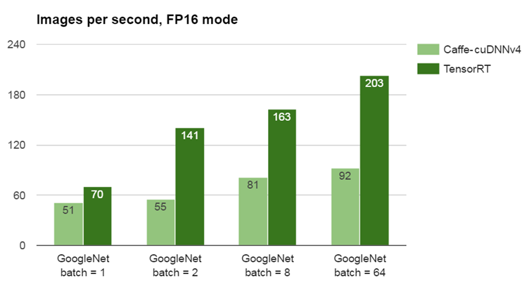
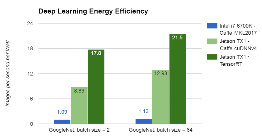
According to the NVIDIA blog introducing TensorRT, the performance improvements brought by TensorRT might swing the comparison in favour of NVIDIA even for small batch sizes: ~18-22 images per second per Watt.
Image(url="https://devblogs.nvidia.com/parallelforall/wp-content/uploads/2016/09/Figure_2-1.png")
Image(url="https://devblogs.nvidia.com/parallelforall/wp-content/uploads/2016/09/Figure_3-1.png")
Collective Knowledge on Deep Learning
Image(url="http://www.engagementaustralia.org.au/blog/wp-content/uploads/2015/03/6-blind-men-hans.jpg")

http://cknowledge.org/ai - crowdsourcing benchmarking and optimisation of AI
System benchmarking and optimisation (this talk)
Model design (future work)
Image(url="https://cdn-images-1.medium.com/max/1000/1*C4Y78hoaN0hPxyWJnkG5vQ.png")
Image(url="https://qiita-image-store.s3.amazonaws.com/0/100523/85381a68-1842-6d2e-e7f2-ced494c6a978.png")

Is it possible to achieve even higher accuracy and better performance?
(Your research here.)
Enabling efficient, reliable and cheap computing - everywhere!
Image(url="http://memecrunch.com/meme/4Z8BF/on-a-mission-from-god/image.jpg")
