Model selection and parameter estimation in dadi
From the tutorial: "∂a∂i is a powerful software tool for simulating the joint frequency spectrum (FS) of genetic variation among multiple populations and employing the FS for population-genetic inference"
Here I will use the dadi Python package to analyze the SFS from RADseq data assembled in pyRAD for three oak species.
## import libraries
import dadi
import numpy as np
import itertools as itt
import pandas as pd
import sys, os

## prettier printing of arrays
pd.set_option('precision',4)
pd.set_option('chop_threshold', 0.001)

## plotting libraries
import matplotlib.pyplot as plt
import seaborn as sns
%matplotlib inline
Convert SNP data to FS
For large data sets fs will be counted from many SNPs and so is easiest to read in from a file. In this case I convert a .loci output file with thousands of RADseq loci from an analysis in pyRAD into the SNP format used by dadi, and then extract the site frequency spectrum from that file.
## a function to select most common element in a list
def most_common(L):
    return max(itt.groupby(sorted(L)),
               key=lambda(x, v):(len(list(v)),
               -L.index(x)))[0]

## a function to get alleles from ambiguous bases
def unstruct(amb):
    " returns bases from ambiguity code"
    D = {"R":["G","A"],
         "K":["G","T"],
         "S":["G","C"],
         "Y":["T","C"],
         "W":["T","A"],
         "M":["C","A"]}
    if amb in D:
        return D.get(amb)
    else:
        return [amb,amb]
## parse the loci
locifile = open("analysis_pyrad/outfiles/virentes_c85d6m4p5.loci")
loci = locifile.read().strip().split("|")
## define focal populations and the outgroups
cuba        = ['CUCA4','CUVN10','CUSV6']
centralA    = ['CRL0030','CRL0001','HNDA09','BZBB1','MXSA3017']
virginiana  = ['FLSF33','FLBA140','SCCU3','LALC2']
geminata    = ["FLCK18","FLSF54","FLWO6","FLAB109"]
minima      = ["FLSF47","FLMO62","FLSA185","FLCK216"]
outgroup    = ["DO","DU","EN","AR","CH","NI","HE","BJSB3","BJVL19","BJSL25"]

## florida is a composite of three 'species'
florida = virginiana+geminata+minima
Projection of data
We are only going to analyze loci that have data for at least 3 individuals in each population, and for at least one outgroup individual. Because we have more samples from Florida we use a minimum of 5 individuals (10 'chromosomes') for this population. The projection is thus [10,6,6], and we use this below to filter the loci down to a list Floci that will be examined.
## minimum samples required to use the locus
proj = [10,6,6]

## only examine loci w/ at least 1 outgroup sample
## and at least two inds from each focal populations
Floci = []   ## filtered locus list
for loc in loci:
    names = [i.strip().split(" ")[0] for i in loc.strip().split("\n")[:-1]]
    if len(set([">"+i for i in outgroup]).intersection(names)) >= 1:
        if len(set([">"+i for i in florida]).intersection(names)) >= proj[0]/2:
            if len(set([">"+i for i in centralA]).intersection(names)) >= proj[1]/2:
                if len(set([">"+i for i in cuba]).intersection(names)) >= proj[2]/2:
                    Floci.append(loc)
Create dadi formatted file
Now we sample from the list of Floci to select a single SNP from each variable locus and write this to a file.
## outfile location
outfile = open("oaks.dadi.snps", 'w')

## print header
print >>outfile, "\t".join(["REF","OUT",
                            "Allele1","fl","ca","cu",
                            "Allele2","fl","ca","cu",
                            "locus","site"])
## recording values
uncalled = 0
calledSNP = 0
uncalledSNP = 0

## iterate over loci
for locN, loc in enumerate(Floci):
    ## to filter a single SNP per locus
    singleSNP = 0

    ## separate names, loci, and SNP identifier line
    names = [i.strip().split(" ")[0] for i in loc.strip().split("\n")[:-1]]
    dat = [i.strip().split(" ")[-1] for i in loc.strip().split("\n")[:-1]]
    snps = loc.strip().split("\n")[-1][14:]

    ## select ingroups v. outgroups
    ihits = [names.index(">"+i) for i in cuba+centralA+florida \
             if ">"+i in names]
    ohits = [names.index(">"+i) for i in outgroup \
             if ">"+i in names]

    ## select a single variable SNP from each locus
    ## but also record how many are skipped for calculating
    ## effective sequence length later
    for site,char in enumerate(snps):
        if char in ["-","*"]:
            ## get common (reference) alleles
            i2 = ["-"+dat[k][site]+"-" for k in ihits if dat[k][site] not in ["N","-"]]
            o2 = ["-"+dat[k][site]+"-" for k in ohits if dat[k][site] not in ["N","-"]]
            ## filter out uninformative sites
            b1 = any([i[1] not in ['N','-'] for i in i2])
            b2 = any([i[1] not in ['N','-'] for i in o2])
            if not (b1 and b2):
                uncalled += 1
            else:
                ## if site is variable in the ingroups
                if len(set(i2)) > 1:
                    ## get the segregating alleles
                    alleles = list(itt.chain(*[unstruct(i[1]) for i in i2]))
                    allele1 = most_common(alleles)
                    allele2 = most_common([i for i in alleles if i!=allele1])
                    outg = most_common(list(itt.chain(*[unstruct(i[1]) for i in o2])))
                    ## florida
                    fl = [names.index(">"+z) for z in florida if ">"+z in names]
                    fldat = list(itt.chain(*[unstruct(dat[z][site]) for z in fl]))
                    fl1,fl2 = fldat.count(allele1), fldat.count(allele2)
                    ## central America
                    ca = [names.index(">"+z) for z in centralA if ">"+z in names]
                    cadat = list(itt.chain(*[unstruct(dat[z][site]) for z in ca]))
                    ca1,ca2 = cadat.count(allele1), cadat.count(allele2)
                    ## cuba
                    cu = [names.index(">"+z) for z in cuba if ">"+z in names]
                    cudat = list(itt.chain(*[unstruct(dat[z][site]) for z in cu]))
                    cu1,cu2 = cudat.count(allele1), cudat.count(allele2)

                    if not singleSNP:
                        calledSNP += 1
                        print >>outfile, "\t".join(map(str,["-"+allele1+"-",
                                                        "-"+outg+"-",
                                                        allele1, fl1, ca1, cu1,
                                                        allele2, fl2, ca2, cu2,
                                                        str(locN), str(site)]))
                        singleSNP = 1
                    else:
                        uncalledSNP += 1

outfile.close()

Nloci = len(Floci)
print "loci\t",Nloci
print "bp\t",Nloci*90
L = Nloci*90-uncalled
print "called bp\t",L
print 'called SNP\t', calledSNP
print 'uncalledSNP\t', uncalledSNP
propcalled = calledSNP/float(calledSNP+uncalledSNP)
print 'prop\t', propcalled
loci	7794
bp	701460
called bp	701161
called SNP	2043
uncalledSNP	836
prop	0.709621396318
The input file looks like this
! head -20 oaks.dadi.snps
REF	OUT	Allele1	fl	ca	cu	Allele2	fl	ca	cu	locus	site
-C-	-C-	C	19	8	6	A	1	0	0	3	56
-G-	-G-	G	15	10	6	A	1	0	0	10	37
-G-	-G-	G	20	6	6	C	2	0	0	23	11
-C-	-A-	C	19	10	5	T	1	0	1	25	25
-T-	-T-	T	13	8	6	C	1	0	0	28	78
-C-	-C-	C	22	7	6	T	0	1	0	32	78
-T-	-T-	T	16	7	6	C	2	1	0	38	65
-T-	-T-	T	18	7	6	C	0	1	0	40	80
-G-	-G-	G	9	8	6	C	13	0	0	42	29
-T-	-T-	T	11	6	6	G	3	0	0	43	84
-T-	-T-	T	10	8	4	C	2	0	0	51	85
-C-	-C-	C	22	9	6	A	0	1	0	53	10
-T-	-T-	T	12	9	6	G	0	1	0	54	28
-T-	-T-	T	16	8	6	C	2	0	0	56	86
-T-	-T-	T	15	8	6	C	1	0	0	65	40
-C-	-C-	C	8	8	6	T	2	0	0	75	68
-C-	-C-	C	11	5	6	G	1	1	0	80	6
-T-	-T-	T	22	10	4	C	0	0	2	81	87
-C-	-C-	C	14	10	6	G	4	0	0	85	10
Convert dadi snps file to SFS
After trying several projections, and with or without corners masked, I settled on the following data set. The projection maximizes data available for the three Cuban samples, and unmasking corners incorporates a significant amount of information about alleles that are fixed between populations, since the populations used here are fairly divergent.
## parse the snps file
dd = dadi.Misc.make_data_dict('oaks.dadi.snps')

## extract the fs from this dict with data not projected
## down to fewer than the total samples
fs = dadi.Spectrum.from_data_dict(dd,
                                  pop_ids=["fl","ca","cu"],
                                  projections=proj,
                                  polarized=True)
## how many segregating sites after projection?
print fs.S()
1626.19720629
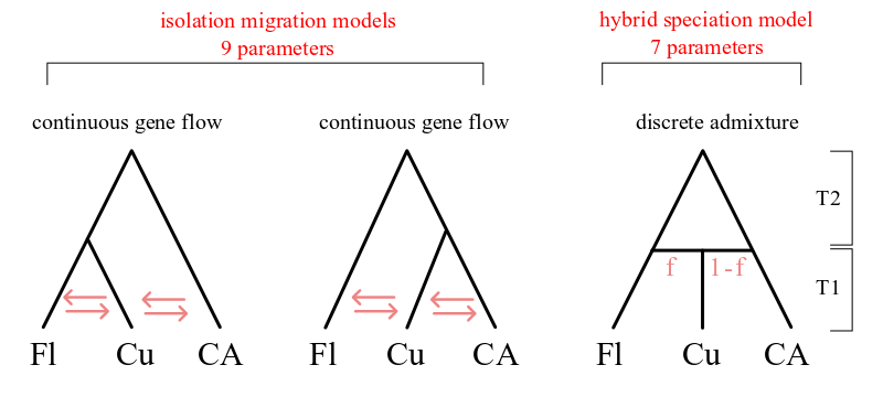
Define three IM-type models
Models IM1 and IM2 are isolation-migration models for a 3 population tree in which Cuba is derived from one lineage or the other. The admix model has the Cuban population formed as an instantaneous fusion of the other two populations, after which it does not exchange gene flow with the parent populations. A separate population size is estimated for each population. Migration is set to zero between Florida and Central America.
Model 1: Island conversion model
## scenario ((florida,cuba),centralA);

def IM_split1(params, ns, pts):
    ## parse params
    N1,N2,N3,T2,T1,m13,m31,m23,m32 = params

    ## create a search grid
    xx = dadi.Numerics.default_grid(pts)

    ## create ancestral pop
    phi = dadi.PhiManip.phi_1D(xx)

    ## split ancestral pop into two species
    phi = dadi.PhiManip.phi_1D_to_2D(xx,phi)

    ## allow drift to occur along each of these branches
    phi = dadi.Integration.two_pops(phi, xx, T2, nu1=N1, nu2=N2, m12=0., m21=0.)

    ## split pop1 into pops 1 and 3
    phi = dadi.PhiManip.phi_2D_to_3D_split_1(xx, phi)

    ## allow drift and migration to occur along these branches
    phi = dadi.Integration.three_pops(phi, xx, T1,
                                       nu1=N1, nu2=N2, nu3=N3,
                                       m12=0.0, m13=m13,
                                       m21=0.0, m23=m23,
                                       m31=m31, m32=m32)
    ## simulate the fs
    fs = dadi.Spectrum.from_phi(phi,ns,(xx,xx,xx),
                                pop_ids=['fl', 'ca', 'cu'])
    return fs
Model 2: Island conversion model
## scenario ((centralA,cuba),florida);

def IM_split2(params, ns, pts):
    ## parse params
    N1,N2,N3,T2,T1,m13,m31,m23,m32 = params

    ## create a search grid
    xx = dadi.Numerics.default_grid(pts)

    ## create ancestral pop
    phi = dadi.PhiManip.phi_1D(xx)

    ## split ancestral pop into two species
    phi = dadi.PhiManip.phi_1D_to_2D(xx,phi)

    ## allow drift to occur along each of these branches
    phi = dadi.Integration.two_pops(phi, xx, T2, nu1=N1, nu2=N2, m12=0., m21=0.)

    ## split pop2 into pops 2 and 3
    phi = dadi.PhiManip.phi_2D_to_3D_split_2(xx, phi)

    ## allow drift and migration to occur along these branches
    phi = dadi.Integration.three_pops(phi, xx, T1,
                                      nu1=N1, nu2=N2, nu3=N3,
                                      m12=0.0, m13=m13,
                                      m21=0.0, m23=m23,
                                      m31=m31, m32=m32)
    ## simulate the fs
    fs = dadi.Spectrum.from_phi(phi,ns,(xx,xx,xx),
                                pop_ids=['fl', 'ca', 'cu'])
    return fs
Model 3: instantaneous admixture
## scenario hybrid speciation forms cuba.

def admix(params, ns, pts):
    ## parse params
    N1,N2,N3,T2,T1,f = params

    ## create a search grid
    xx = dadi.Numerics.default_grid(pts)

    ## make ancestral pop that splits into two
    phi = dadi.PhiManip.phi_1D(xx)
    phi = dadi.PhiManip.phi_1D_to_2D(xx,phi)

    ## allow drift to occur along each of these branches
    phi = dadi.Integration.two_pops(phi, xx, T2, nu1=N1, nu2=N2, m12=0., m21=0.)

    ## create pop 3 from a mixture of 1 and 2
    phi = dadi.PhiManip.phi_2D_to_3D_admix(phi, f, xx, xx, xx)

    ## allow drift and migration to occur along these branches
    ## cuba population shrinks in size after divergence
    phi = dadi.Integration.three_pops(phi, xx, T1,
                                      nu1=N1, nu2=N2, nu3=N3,
                                      m12=0.0, m13=0.0,
                                      m21=0.0, m23=0.0,
                                      m31=0.0, m32=0.0)
    ## simulate the fs
    fs = dadi.Spectrum.from_phi(phi,ns,(xx,xx,xx),
                                pop_ids=['fl', 'ca', 'cu'])
    return fs
## sample sizes
ns = fs.sample_sizes

## points used for exrapolation
pts_l = [12, 20, 32]

## starting values for params
N1 = N2 = N3 = 2.0
T2 = 2.0
T1 = 2.0
m13 = m31 = m23 = m32 = 0.1
f  = 0.4999

## create starting parameter sets
params_IM    = np.array([N1,N2,N3,T2,T1,m13,m31,m23,m32])
params_admix = np.array([N1,N2,N3,T2,T1,f])

## search limits
upper_IM    = [10.0,10.0,10.0, 10.0,10.0, 25.0, 25.0, 25.0, 25.0]
lower_IM    = [1e-3,1e-3,1e-3, 1e-3,1e-3, 1e-5, 1e-5, 1e-5, 1e-5]

upper_admix = [10.0,10.0,10.0, 10.0,10.0, 0.9999]
lower_admix = [1e-3,1e-3,1e-3, 1e-3,1e-3, 0.0001]
Python script for model fitting
I wrote a separate Python script for each model in which the parameters were estimated using the commands below. This was done 10 times for each model from different starting positions. These were executed in separate Python shells because optimization sometimes freezes in bad parameter space, and because it allowed easy parallelization. These scripts are available in the git repository as dadi_m1X.py, dadi_m2X.py, and dadi_m3X.py.
%%bash
## example of running code
## python analysis_dadi/dadi_m1X.py
#### Example code for optimization in script dadi_m1X.py
## model = IM_split1
## params= params_IM
## uppers= upper_IM
## lowers= lower_IM
## maxiters=10

#### Create extrapolating function
## Func = dadi.Numerics.make_extrap_log_func(model)

#### Perturb start values
## p0 = dadi.Misc.perturb_params(params, fold=2.,
##                              upper_bound=uppers,
##                              lower_bound=lowers)

#### optimize from starting position
## args = [p0, fs, Func, pts_l, lowers, uppers, 0, maxiters]
## popt = dadi.Inference.optimize_log_lbfgsb(*args)

#### return the likelihood of the data under these parameters
## mod = Func(popt, ns, pts_l)
## ll_opt = dadi.Inference.ll_multinom(mod, fs)
Optimized best fit from 10 random starting positions
## optimized at projection (10,6,6); extrap (12,20,32); S=1626
ml1 = [2.5013156716397473, 0.68871161421841698, 0.076807020757753017,
       0.70851628972828207, 0.14901468477012897, 0.14349173980106683,
       12.58678666702065, 1.2625236526206685, 21.036230092460865, -543.08153591196356]

ml2 = [2.412336866389539, 0.66060145092919675, 0.23061219403870617,
       0.71073109877391338, 0.084218967415615298, 0.138041546493126,
       6.036453130870238, 4.09467065466802, 0.0031179372963987696, -541.90248015938994]

ml3 = [2.2562645699939852, 0.71705301735090954, 0.14307134998023263,
       0.57976328038133673, 0.025790751880146609, 0.38345451331222341,
       -555.34376821105138]
indexnames = ["N1","N2","N3","T2","T1","m13","m31","m23","m32","LL"]
ML1 = pd.Series(ml1, index = indexnames)
ML2 = pd.Series(ml2, index = indexnames)
ML3 = pd.Series(ml3, index=["N1","N2","N3","T2","T1","f","LL"])
data = pd.DataFrame([ML1,ML2,ML3],index=["ML1","ML2","ML3"]).T
print data
         ML1      ML2      ML3
LL  -543.082 -541.902 -555.344
N1     2.501    2.412    2.256
N2     0.689    0.661    0.717
N3     0.077    0.231    0.143
T1     0.149    0.084    0.026
T2     0.709    0.711    0.580
f        NaN      NaN    0.383
m13    0.143    0.138      NaN
m23    1.263    4.095      NaN
m31   12.587    6.036      NaN
m32   21.036    0.003      NaN

[11 rows x 3 columns]
## optimized grid
pts_l = [12,20,32]

# The optimal value of theta given the model.
Func = dadi.Numerics.make_extrap_log_func(IM_split1)
model1_AFS = Func(ML1.tolist()[:-1],ns,pts_l)
theta1 = dadi.Inference.optimal_sfs_scaling(model1_AFS, fs)

# The optimal value of theta given the model.
Func = dadi.Numerics.make_extrap_log_func(IM_split2)
model2_AFS = Func(ML2.tolist()[:-1],ns,pts_l)
theta2 = dadi.Inference.optimal_sfs_scaling(model2_AFS, fs)

# The optimal value of theta given the model.
Func = dadi.Numerics.make_extrap_log_func(admix)
model3_AFS = Func(ML3.tolist()[:-1],ns,pts_l)
theta3 = dadi.Inference.optimal_sfs_scaling(model3_AFS, fs)
ML estimates in converted units
###### Fixed params
mu = 2.5e-9         ## from Populus article by xxyy
gentime = 30.0   ## (years) from Gugger & Cavender-Bares

models = [ML1,ML2,ML3]
thetas = [theta1,theta2,theta3]
for model,theta in zip(models,thetas):
    print "\n-----model %s-------" % str(thetas.index(theta)+1)
    ## Population sizes
    Nref = theta/(4*mu*L)
    print "theta =\t",theta, "("+str(theta/Nloci)+")"
    print "Nref =\t",round(Nref)
    print "N1 =\t",round(Nref*model["N1"])
    print "N2 =\t",round(Nref*model["N2"])
    print "N3 =\t",round(Nref*model["N3"])
    ## Divergence times
    T1  = model["T1"]
    T12 = model["T1"] + model["T2"]
    print 'T1  =\t',round( ( T1*2*Nref * gentime)/1e6, 3), 'Mya'
    print 'T12 =\t',round( (T12*2*Nref * gentime)/1e6, 3), 'Mya'
    ## Migration
    if 'f' in model.index:
        print 'f   =\t', model['f']
        print '1-f =\t', 1-(model["f"])
    else:
        print 'm13 =\t', (model["m13"])/(2*Nref) * 1e3
        print 'm31 =\t', (model["m31"])/(2*Nref) * 1e3
        print 'm23 =\t', (model["m23"])/(2*Nref) * 1e3
        print 'm32 =\t', (model["m32"])/(2*Nref) * 1e3
-----model 1-------
theta =	249.587274958 (0.0320230016626)
Nref =	35596.0
N1 =	89038.0
N2 =	24516.0
N3 =	2734.0
T1  =	0.318 Mya
T12 =	1.831 Mya
m13 =	0.00201554369684
m31 =	0.176799156281
m23 =	0.0177339238738
m32 =	0.295483496311

-----model 2-------
theta =	256.759934829 (0.0329432813484)
Nref =	36619.0
N1 =	88338.0
N2 =	24191.0
N3 =	8445.0
T1  =	0.185 Mya
T12 =	1.747 Mya
m13 =	0.00188482188323
m31 =	0.0824218450692
m23 =	0.0559087104615
m32 =	4.25723747386e-05

-----model 3-------
theta =	282.456200226 (0.0362402104472)
Nref =	40284.0
N1 =	90892.0
N2 =	28886.0
N3 =	5763.0
T1  =	0.062 Mya
T12 =	1.464 Mya
f   =	0.383454513312
1-f =	0.616545486688
plt.rcParams['figure.figsize'] = (6,6)
dadi.Plotting.plot_3d_comp_multinom(model1_AFS, fs, vmin=0.1, resid_range=3,
                                    pop_ids =('fl', 'ca', 'cu'))

Model 2
plt.rcParams['figure.figsize'] = (6,6)
dadi.Plotting.plot_3d_comp_multinom(model2_AFS, fs, vmin=0.1, resid_range=3,
                                    pop_ids =('fl', 'ca', 'cu'))

<matplotlib.figure.Figure at 0x1087eb90>
Model 3
plt.rcParams['figure.figsize'] = (6,6)
dadi.Plotting.plot_3d_comp_multinom(model3_AFS, fs, vmin=0.1, resid_range=3,
                                    pop_ids =('fl', 'ca','cu'))

Parametric bootstrapping from simulated data in ms.
We generate simulated data sets under the same demographic scenarios as in the dadi models. We save each of the simulated data sets because these will also be used for model selection below.
Functions for simulating data in ms
#############################################################
### IM_split 1
def simSFS_model1(theta, N1,N2,N3,mig,T1, T12):
    R1,R2,R3 = np.random.random_integers(0,9999999,3)
    command = """ ms 22 7794 \
                     -t %(theta)f \
                     -I 3 10 6 6 \
                     -n 1 %(N1)f \
                     -n 2 %(N2)f \
                     -n 3 %(N3)f \
                     -en %(T1)f 1 %(N1)f \
                     -ma %(mig)s \
                     -ej %(T1)f 3 1 \
                     -ej %(T12)f 2 1 \
                     -en %(T12)f 1 1 \
                     -seeds %(R1)f %(R2)f %(R3)f """
    sub_dict = {'theta':theta, 'N1':N1, 'N2':N2, 'N3':N3,
                'T1':T1, 'mig':" ".join(mig),
                'R1':R1, 'R2':R2, 'R3':R3}
    mscommand = command % sub_dict
    fs = dadi.Spectrum.from_ms_file(os.popen(mscommand), average=False)
    return fs

###############################################################
## IM_split 2
def simSFS_model2(theta, N1,N2,N3,mig,T1, T12):
    R1,R2,R3 = np.random.random_integers(0,9999999,3)
    command = """ ms 22 7794 \
                     -t %(theta)f \
                     -I 3 10 6 6 \
                     -n 1 %(N1)f \
                     -n 2 %(N2)f \
                     -n 3 %(N3)f \
                     -en %(T1)f 2 %(N2)f \
                     -ma %(mig)s \
                     -ej %(T1)f 3 2 \
                     -ej %(T12)f 2 1 \
                     -en %(T12)f 1 1 \
                     -seeds %(R1)f %(R2)f %(R3)f """
    sub_dict = {'theta':theta, 'N1':N1, 'N2':N2, 'N3':N3,
                'T1':T1, 'mig':" ".join(mig),
                'R1':R1, 'R2':R2, 'R3':R3}
    mscommand = command % sub_dict
    fs = dadi.Spectrum.from_ms_file(os.popen(mscommand), average=False)
    return fs

#################################################################
## Admix
def simSFS_model3(theta, N1,N2,N3,T1, T12,f):
    R1,R2,R3 = np.random.random_integers(0,9999999,3)
    command = """ ms 22 7794 \
                     -t %(theta)f \
                     -I 3 10 6 6 \
                     -n 1 %(N1)f \
                     -n 2 %(N2)f \
                     -n 3 %(N3)f \
                     -en %(T1)f 2 %(N2)f \
                     -en %(T1)f 1 %(N1)f \
                     -es %(T1)f 3 %(f)f \
                     -ej %(T1)f 4 2 \
                     -ej %(T1)f 3 1 \
                     -ej %(T12)f 2 1 \
                     -en %(T12)f 1 1 \
                     -seeds %(R1)f %(R2)f %(R3)f """
    sub_dict = {'theta':theta, 'N1':N1, 'N2':N2, 'N3':N3,
                'T1':T1, 'f':f,
                'R1':R1, 'R2':R2, 'R3':R3}
    mscommand = command % sub_dict
    fs = dadi.Spectrum.from_ms_file(os.popen(mscommand), average=False)
    return fs
Estimated parameters
Execute Python scripts with the above code in a separate shell
This creates 200 parametric bootstrap data sets for each of the three models, and re-estimates parameters under each of the three models. The sfs for each bootstrap data set is saved in a directory called pboots/. The Python scripts to execute this are in the git repository as dadi_m1boot_fit3.py, dadi_m2boot_fit3.py, and dadi_m3boot_fit3.py. Nine output files were created and in are in the git repo. For example, the optimized parameters for a data set simulated under model 1 and fit using model 2 is saved to the file dadi_m1_f2_boots.txt.
%%bash
## commented out b/c it takes a long time to run

## for i in $(seq 1 200);
##   do python analysis_dadi/dadi_m1boot_fit3.py
## done

## for i in $(seq 1 200);
##   do python analysis_dadi/dadi_m2boot_fit3.py
## done

## for i in $(seq 1 100);
##   do python analysis_dadi/dadi_m3boot_fit3.py
## done
Calculate biased-corrected confidence intervals
###### Fixed params
mu = 2.5e-9         ## from Populus genome article
gentime = 30.0     ## (years) from Gugger & Cavender-Bares

def makedict(bootfile, theta):
    ## parse file
    DD = {}
    infile = open(bootfile).readlines()
    lines = [i.strip().split("\t") for i in infile]
    bootorder = [int(i[0].replace("boot","")) for i in lines]
    elements = ["N1","N2","N3","T2","T1"]
    for el,li in zip(elements, range(1,6)):
        DD[el] = [float(i[li]) for i in lines]
    if len(lines[0]) > 8:
        elements = ["m13","m31","m23","m32","LL"]
        for el,li in zip(elements, range(6,11)):
            DD[el] = [float(i[li]) for i in lines]
    else:
        DD['f'] = [float(i[6]) for i in lines]
        DD['LL'] = [float(i[7]) for i in lines]
    DD['sLL'] = [DD["LL"][i-1] for i in bootorder[:60]]
    return DD
Model 1
DD = makedict("analysis_dadi/dadi_m1_f1_boots.txt", theta1)

#############################
Nref = theta1/(4*mu*L)
#############################

print "Model 1"
for param in ["N1","N2","N3"]:
    m = np.mean([(i*Nref) for i in DD[param]])
    s = np.std([(i*Nref) for i in DD[param]])
    o = (ML1[param]*Nref)
    unbiased = o-(m-o)
    print param, max(0,unbiased-1.96*s), o, unbiased+1.96*s

#############################
m = np.mean([(i*Nref*2*gentime)/1e6 for i in DD["T1"]])
s = np.std([(i*Nref*2*gentime)/1e6 for i in DD["T1"]])
o = (ML1["T1"]*Nref*2*gentime)/1e6
unbiased = o-(m-o)
print "T1", max(0,unbiased-1.96*s), o, unbiased+1.96*s
m = np.mean([(i*Nref*2*gentime)/1e6 for i in (DD["T1"]+DD["T2"])])
s = np.std([(i*Nref*2*gentime)/1e6 for i in (DD["T1"]+DD["T2"])])
o = ((ML1["T1"]+ML1["T2"])*Nref*2*gentime)/1e6
unbiased = o-(m-o)
print "T12", max(0,unbiased-1.96*s), o, unbiased+1.96*s


#############################
for param in ["m13","m31","m23","m32"]:
    m = np.mean([i/(2*Nref) for i in DD[param]])
    s = np.std([i/(2*Nref) for i in DD[param]])
    o = (ML1[param]/(2*Nref))
    unbiased = o-(m-o)
    print param, max(0,(unbiased-1.96*s)*1e3), o*1e3, (unbiased+1.96*s)*1e3

m = np.mean(DD["LL"])
s = np.std(DD["LL"])
o = ML1["LL"]
unbiased = o-(m-o)
print "LL", m-1.96*s, o, m+1.96*s
Model 1
N1 71475.9003173 89037.5480517 100269.854037
N2 18585.0359322 24515.5755989 29469.4608854
N3 0 2734.04467855 5301.53276347
T1 0 0.318262160336 0.896697430149
T12 1.43013516666 1.8314950699 3.99576741889
m13 0 0.00201554369684 0.00779580837604
m31 0.0204317889296 0.176799156281 0.338742961336
m23 0.00280410835358 0.0177339238738 0.0298659118644
m32 0.0155455991765 0.295483496311 0.519561371751
LL -611.90667302 -543.081535912 -547.307616243
Model 2
DD = makedict("analysis_dadi/dadi_m2_f2_boots.txt", theta2)

#############################
Nref = theta2/(4*mu*L)
#############################
print "Model 2"
for param in ["N1","N2","N3"]:
    m = np.mean([(i*Nref) for i in DD[param]])
    s = np.std([(i*Nref) for i in DD[param]])
    o = (ML2[param]*Nref)
    unbiased = o-(m-o)
    print param, max(0,unbiased-1.96*s), o, unbiased+1.96*s

#############################
m = np.mean([(i*Nref*2*gentime)/1e6 for i in DD["T1"]])
s = np.std([(i*Nref*2*gentime)/1e6 for i in DD["T1"]])
o = (ML2["T1"]*Nref*2*gentime)/1e6
unbiased = o-(m-o)
print "T1", max(0,unbiased-1.96*s), o, unbiased+1.96*s
m = np.mean([(i*Nref*2*gentime)/1e6 for i in (DD["T1"]+DD["T2"])])
s = np.std([(i*Nref*2*gentime)/1e6 for i in (DD["T1"]+DD["T2"])])
o = ((ML2["T1"]+ML2["T2"])*Nref*2*gentime)/1e6
unbiased = o-(m-o)
print "T12", max(0,unbiased-1.96*s), o, unbiased+1.96*s


#############################
for param in ["m13","m31","m23","m32"]:
    m = np.mean([i/(2*Nref) for i in DD[param]])
    s = np.std([i/(2*Nref) for i in DD[param]])
    o = (ML2[param]/(2*Nref))
    unbiased = o-(m-o)
    print param, max(0,(unbiased-1.96*s)*1e3), o*1e3, (unbiased+1.96*s)*1e3

m = np.mean(DD["LL"])
s = np.std(DD["LL"])
o = ML2["LL"]
unbiased = o-(m-o)
#print "LL", unbiased-1.96*s, o, unbiased+1.96*s
print "LL", m-1.96*s, o, m+1.96*s
Model 2
N1 69722.5763103 88337.9789521 100024.420796
N2 17818.7840481 24190.7330112 29340.4289636
N3 2379.47192323 8444.84674878 13458.644633
T1 0.0363476312861 0.185042150819 0.305737745991
T12 1.18583067533 1.74662875306 3.99630587332
m13 0 0.00188482188323 0.00472397460442
m31 0.00752720476581 0.0824218450692 0.148066108791
m23 0.0242008829239 0.0559087104615 0.0867269369484
m32 0 4.25723747386e-05 0.00426563585615
LL -605.553218248 -541.902480159 -542.596028013
Model 3
DD = makedict("analysis_dadi/dadi_m3_f3_boots.txt", theta2)

#############################
Nref = theta3/(4*mu*L)
#############################
print "Model 3"
for param in ["N1","N2","N3"]:
    m = np.mean([(i*Nref) for i in DD[param]])
    s = np.std([(i*Nref) for i in DD[param]])
    o = (ML3[param]*Nref)
    unbiased = o-(m-o)
    print param, max(0,unbiased-1.96*s), o, unbiased+1.96*s

#############################
m = np.mean([(i*Nref*2*gentime)/1e6 for i in DD["T1"]])
s = np.std([(i*Nref*2*gentime)/1e6 for i in DD["T1"]])
o = (ML3["T1"]*Nref*2*gentime)/1e6
unbiased = o-(m-o)
print "T1", max(0,unbiased-1.96*s), o, unbiased+1.96*s
m = np.mean([(i*Nref*2*gentime)/1e6 for i in (DD["T1"]+DD["T2"])])
s = np.std([(i*Nref*2*gentime)/1e6 for i in (DD["T1"]+DD["T2"])])
o = ((ML3["T1"]+ML3["T2"])*Nref*2*gentime)/1e6
unbiased = o-(m-o)
print "T12", max(0,unbiased-1.96*s), o, unbiased+1.96*s


#############################
m = np.mean(DD["f"])
s = np.std(DD["f"])
o = (ML3['f'])
unbiased = o-(m-o)
print 'f', unbiased-1.96*s, o, unbiased+1.96*s

m = np.mean(DD["LL"])
s = np.std(DD["LL"])
o = ML3["LL"]
unbiased = o-(m-o)
print "LL", m-1.96*s, o, m+1.96*s
Model 3
N1 70873.444192 90891.5237933 104798.634546
N2 22628.9371512 28885.8151896 33641.5723239
N3 342.65514223 5763.49652599 10702.788427
T1 0.00234647793955 0.0623373899321 0.114684927723
T12 0.805824744774 1.46365092454 3.53834571718
f 0.337902679016 0.383454513312 0.417653307748
LL -632.794946497 -555.343768211 -566.776149859
Report 95% range of LL
DD = makedict("dadi_m1_f3_boots.txt", theta2)
m = np.mean(DD["LL"])
s = np.std(DD["LL"])
o = ML1["LL"]
print "LL", m-1.96*s, o, m+1.96*s
LL -629.472792108 -543.081535912 -562.55636251
DD = makedict("dadi_m1_f2_boots.txt", theta2)
m = np.mean(DD["LL"])
s = np.std(DD["LL"])
o = ML1["LL"]
print "LL", m-1.96*s, o, m+1.96*s
LL -618.44626393 -543.081535912 -550.43080575
DD = makedict("dadi_m2_f1_boots.txt", theta2)
m = np.mean(DD["LL"])
s = np.std(DD["LL"])
o = ML2["LL"]
print "LL", m-1.96*s, o, m+1.96*s
LL -610.625740669 -541.902480159 -548.678268059
DD = makedict("dadi_m2_f3_boots.txt", theta2)
m = np.mean(DD["LL"])
s = np.std(DD["LL"])
o = ML2["LL"]
print "LL", m-1.96*s, o, m+1.96*s
LL -626.694918671 -541.902480159 -562.578122564
DD = makedict("dadi_m3_f1_boots.txt", theta2)
m = np.mean(DD["LL"])
s = np.std(DD["LL"])
o = ML3["LL"]
print "LL", m-1.96*s, o, m+1.96*s
LL -633.253767231 -555.343768211 -568.236956872
DD = makedict("dadi_m3_f2_boots.txt", theta2)
m = np.mean(DD["LL"])
s = np.std(DD["LL"])
o = ML3["LL"]
print "LL", m-1.96*s, o, m+1.96*s
LL -638.846613236 -555.343768211 -571.185797893
Monte Carlo model selection:
Compare the area of overlap of log-likelihood ratio statistics $\delta$
$\delta$ = -2(log L$_2$ - log L$_1$)
following Boettiger et al. (2012)
Can we reject the simplest model (model 3)?
Let's begin by assuming that model 3 is true (the null model). We ask how does the observed difference in log likelihoods for the fit of our empirical data to the two models ($\delta_{32}$ and $\delta_{31}$) compare to the difference in log likelihood fits when the data are simulated under model 3 ($\delta_{32sim3}$, $\delta_{31sim3}$)?
delta32obs = -2.*(ML3["LL"] - ML2["LL"])
delta31obs = -2.*(ML3["LL"] - ML1["LL"])

print 'LL model3:', ML3["LL"]
print 'LL model2:', ML2["LL"]
print 'LL model1:', ML1["LL"]
print 'delta32 observed:', delta32obs
print 'delta31 observed:', delta31obs
LL model3: -555.343768211
LL model2: -541.902480159
LL model1: -543.081535912
delta32 observed: 26.8825761033
delta31 observed: 24.5244645982
Read in the optimized bootstrap fits.
W = ['title','N1','N2','N3','T2','T1','m13','m31','m23','m32','LL']
LL31 = pd.read_table("dadi_m3_f1_boots.txt", sep="\t", names=W, index_col=0).sort()["LL"]

W = ['title','N1','N2','N3','T2','T1','m13','m31','m23','m32','LL']
LL32 = pd.read_table("dadi_m3_f2_boots.txt", sep="\t", names=W, index_col=0).sort()["LL"]

W = ['title','N1','N2','N3','T2','T1','f','LL']
LL33 = pd.read_table("dadi_m3_f3_boots.txt", sep="\t", names=W, index_col=0).sort()["LL"]
Measure the distribution of LL differences on data simulated under model 3
delta32sim3 = -2.*(LL33-LL32)
delta31sim3 = -2.*(LL33-LL31)
Plot the observed and simulated LL differences between models
plt.rcParams['figure.figsize'] = (6,4)

sns.kdeplot(delta32sim3, shade=True, label="$\delta_{32}$")
sns.kdeplot(delta31sim3, shade=True, label="$\delta_{31}$")
sns.despine()

plt.vlines(delta32obs, 0, 0.05, lw=3, color='#262626',
           label='$\delta_{32obs}$', linestyles='dashed')
plt.vlines(delta31obs, 0, 0.05, lw=3, color='#F65655',
           label='$\delta_{31obs}$', linestyles='dashed')
plt.title("model 3 sims")
plt.legend(loc=2)
<matplotlib.legend.Legend at 0x22dad090>

Is the difference significantly outside the expectation?
The proportion of sims greater than the observed delta values is 0. This is effectively a P-value for the probability that a difference at least this large would be seen under model 3. A more accurate way, though, is to calculate $\delta^*$, the upper 95% or 99% percentile of the simulated distribution, and ask if our observed delta is greater than this.
delta32star = np.percentile(delta32sim3, 99)
delta31star = np.percentile(delta31sim3, 99)
print 'delta32star', delta32star
print 'delta31star', delta31star
print 'deltaobs', delta32obs
delta32star 3.907066664
delta31star 9.00921333
deltaobs 26.8825761033
Can we reject model 3 for either of the more complex models?
At a false positive rate of 0.05, Yes definitely, because observed $\delta$ >> $\delta^*$
print delta32obs > delta32star
print delta31obs > delta31star
True
True
Power to reject model 3
We next need to ask what is the probability that we correctly reject model 3 when the data comes from model 2 or model 1? This is a concern because the greater complexity of these models will bias us towards usually thinking they are better.
Load bootstrap data simulated under model 2.
W = ['title','N1','N2','N3','T2','T1','m13','m31','m23','m32','LL']
LL21 = pd.read_table("dadi_m2_f1_boots.txt", sep="\t", names=W, index_col=0).sort()["LL"]

W = ['title','N1','N2','N3','T2','T1','m13','m31','m23','m32','LL']
LL22 = pd.read_table("dadi_m2_f2_boots.txt", sep="\t", names=W, index_col=0).sort()["LL"]

W = ['title','N1','N2','N3','T2','T1','f','LL']
LL23 = pd.read_table("dadi_m2_f3_boots.txt", sep="\t", names=W, index_col=0).sort()["LL"]
Calculate $\delta_{32}$ under model 2 sims
delta32sim2 = -2.*(LL23-LL22)
Compare $\delta_{32}$ simulated under both models
plt.rcParams['figure.figsize'] = (6,4)
plt.gcf().subplots_adjust(bottom=0.20, left=0.15)

sns.set_style("ticks")
sns.set_context("paper", font_scale=1.8, rc={"lines.linewidth": 2})
sns.kdeplot(delta32sim2, shade=True, color="#898989",label='$\delta_{sim2}$')
sns.kdeplot(delta32sim3, shade=True, color="#262626", label='$\delta_{sim3}$')
sns.axlabel('Log Likelihood ratio ($\delta$)', 'Density')
sns.despine()

#plt.vlines(delta32star, 0, 0.061, lw=3, color="#262626",
#           linestyles='dashed', label="$\delta^{*}$")
plt.vlines(delta32obs, 0, 0.061, lw=3, color='#F65655',
           linestyles='dashed', label='$\delta_{obs}$')
plt.legend(loc=1)
plt.title("(B) models 2 vs. 3")
plt.savefig("delta32.png", dpi=300)
plt.savefig("delta32.svg")

Calculate % overlap
Our power to reject model 3 is measured by the proportion of the simulations under model 2 that are to the left of the critical delta32star from data simulated under model 3. Remember this value is the 95 percentile of the model 3 bootstraps (0.05 significance), and at this level we find we have 100% power to reject model 3 when model 2 is true (no overlap).
1.-sum(delta32sim2 < delta32star)/float(len(delta32sim2))
1.0
Now the same comparison against model 1
Load bootstrap data simulated under model 1
W = ['title','N1','N2','N3','T2','T1','m13','m31','m23','m32','LL']
LL11 = pd.read_table("dadi_m1_f1_boots.txt", sep="\t", names=W, index_col=0).sort()["LL"]

W = ['title','N1','N2','N3','T2','T1','m13','m31','m23','m32','LL']
LL12 = pd.read_table("dadi_m1_f2_boots.txt", sep="\t", names=W, index_col=0).sort()["LL"]

W = ['title','N1','N2','N3','T2','T1','f','LL']
LL13 = pd.read_table("dadi_m1_f3_boots.txt", sep="\t", names=W, index_col=0).sort()["LL"]
Calculate $\delta_{31}$ under model 1 sims
delta31sim1 = -2.*(LL13-LL11)
Compare $\delta_{31}$ simulated under both models
plt.rcParams['figure.figsize'] = (6,4)
plt.gcf().subplots_adjust(bottom=0.20, left=0.15)

sns.set_style("ticks")
sns.set_context("paper", font_scale=1.8, rc={"lines.linewidth": 2})
sns.kdeplot(delta31sim1, shade=True, color="#898989",label='$\delta_{sim1}$')
sns.kdeplot(delta31sim3, shade=True, color="#262626", label='$\delta_{sim3}$')
sns.axlabel('Log Likelihood ratio ($\delta$)', 'Density')
sns.despine()

plt.vlines(delta31obs, 0, 0.085, lw=3, color='#F65655',
           linestyles='dashed', label='$\delta_{obs}$')
plt.legend(loc=1)
plt.title("(A) models 1 vs. 3")
plt.savefig("delta31.png", dpi=300)
plt.savefig("delta31.svg")

Calculate % overlap
Our power to reject model 3 is measured by the proportion of the simulations under model 1 that are to the left of the critical delta31star from data simulated under model 3. Remember this value is the 95 percentile of the model 3 bootstraps (0.05 significance), and at this level we find we have 92% power to reject model 3 when model 1 is true (no overlap).
1.-sum(delta31sim1 < delta31star)/float(len(delta31sim1))
0.99004975124378114
Compare models 2 & 1
We'll begin by assuming model 1 is the true model. We can see already that the difference between models 2 and 1 is much smaller than it was between 2 and 3. But model 2 is a slightly better fit to the empirical data.
delta12obs = -2.*(ML1["LL"] - ML2["LL"])
delta13obs = -2.*(ML1["LL"] - ML3["LL"])

print 'LL model3:', ML3["LL"]
print 'LL model2:', ML2["LL"]
print 'LL model1:', ML1["LL"]
print 'delta12 observed:', delta12obs
print 'delta13 observed:', delta13obs
LL model3: -555.343768211
LL model2: -541.902480159
LL model1: -543.081535912
delta12 observed: 2.35811150515
delta13 observed: -24.5244645982
How much better?
We compare the difference in their fit to the real data to the difference between them when data is simulated under model 1.
delta12sim1 = -2.*(LL11-LL12)
Is our observed $\delta$ > 95% of the bootstrap values simulated under model 1?
Not quite, but we can reject model 1 in favor of model 2 at a P-value of 0.07.
print 'obs=', delta12obs
delta12star = np.percentile(delta12sim1, 95)
print '\ndelta*95=',delta12star
print delta12obs > delta12star
delta12star = np.percentile(delta12sim1, 94)
print '\ndelta*94=',delta12star
print delta12obs > delta12star
delta12star = np.percentile(delta12sim1, 93)
print '\ndelta*93=',delta12star
print delta12obs > delta12star
obs= 2.35811150515

delta*95= 3.257462352
False

delta*94= 2.603696052
False

delta*93= 1.47879285
True
Calculate $\delta_{12}$ under model 2 sims
delta12sim2 = -2.*(LL21-LL22)
Compare $\delta_{12}$ simulated under both models
plt.rcParams['figure.figsize'] = (6,4)
plt.gcf().subplots_adjust(bottom=0.20, left=0.15)

sns.set_context("paper", font_scale=1.8, rc={"lines.linewidth": 2})
sns.kdeplot(delta12sim1, shade=True, color="#262626", label='$\delta_{sim1}$')
sns.kdeplot(delta12sim2, shade=True, color="#898989", label='$\delta_{sim2}$')

sns.axlabel('Log Likelihood ratio ($\delta$)', 'Density')
sns.despine()

plt.vlines(delta12obs, 0, 0.055, lw=3, color='#F65655',
           linestyles='dashed', label='$\delta_{obs}$')

plt.legend(loc=2)
plt.title("(C) models 1 vs. 2")
plt.savefig("delta12.png", dpi=300)
plt.savefig("delta12.svg")

Calculate % overlap and power
Our power to reject model 1 when model 2 at 0.05 false positive rate is only 85%, given our data.
sum(delta12sim2 > delta12star)/float(len(delta12sim2))
0.85572139303482586