DaCosta & Sorenson (2016) single-end dd-RAD data set
Here we demonstrate a denovo assembly for an empirical RAD data set using the ipyrad Python API. This example was run on a workstation with 20 cores available and takes about <10 minutes to run completely, but can be run on even a laptop in about less than an hour.
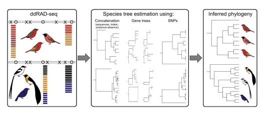
We will use the Lagonosticta and Vidua data set from DaCosta & Sorenson 2016. This data set is composed of single-end 101bp reads from a ddRAD-seq library prepared with the SbfI and EcoRI enzymes and is available on NCBI by its study accession SRP059199. At the end of this notebook we also demonstrate the use of ipyrad.analysis tools to run downstream analyses on this data set.
The figure below from this paper shows the general workflow in which two fairly distinct clades were sequenced together but then analyzed separately.
Setup (software and data files)
If you haven't done so yet, start by installing ipyrad using conda (see ipyrad installation instructions) as well as the packages in the cell below. This is easiest to do in a terminal. Then open a jupyter-notebook, like this one, and follow along with the tutorial by copying and executing the code in the cells, and adding your own documentation between them using markdown. Feel free to modify parameters to see their effects on the downstream results.
## conda install ipyrad -c ipyrad
## conda install toytree -c eaton-lab
## conda install entrez-direct -c bioconda
## conda install sratools -c bioconda
## imports
import ipyrad as ip
import ipyrad.analysis as ipa
import ipyparallel as ipp
In contrast to the ipyrad CLI, the ipyrad API gives users much more fine-scale control over the parallelization of their analysis, but this also requires learning a little bit about the library that we use to do this, called ipyparallel. This library is designed for use with jupyter-notebooks to allow massive-scale multi-processing while working interactively.
Understanding the nuts and bolts of it might take a little while, but it is fairly easy to get started using it, especially in the way it is integrated with ipyrad. To start a parallel client to you must run the command-line program 'ipcluster'. This will essentially start a number of independent Python processes (kernels) which we can then send bits of work to do. The cluster can be stopped and restarted independently of this notebook, which is convenient for working on a cluster where connecting to many cores is not always immediately available.
Open a terminal and type the following command to start an ipcluster instance with N engines.
## ipcluster start --n=20
## connect to cluster
ipyclient = ipp.Client()
ipyclient.ids
[0, 1, 2, 3, 4, 5, 6, 7, 8, 9, 10, 11, 12, 13, 14, 15, 16, 17, 18, 19]
Download the data set (Finches)
These data are archived on the NCBI sequence read archive (SRA) under accession id SRP059199. For convenience, the data are also hosted at a public Dropbox link which is a bit easier to access. Run the code below to download and decompress the fastq data files, which will save them into a directory called fastqs-Finches/.
## download the Pedicularis data set from NCBI
sra = ipa.sratools(accession="SRP059199", workdir="fastqs-Finches")
sra.run(force=True, ipyclient=ipyclient)
[####################] 100%  Downloading fastq files | 0:00:52 |
24 fastq files downloaded to /home/deren/Documents/ipyrad/tests/fastqs-Finches
Create an Assembly object
This object stores the parameters of the assembly and the organization of data files.
## you must provide a name for the Assembly
data = ip.Assembly("Finches")
New Assembly: Finches
Set parameters for the Assembly. This will raise an error if any of the parameters are not allowed because they are the wrong type, or out of the allowed range.
## set parameters
data.set_params("project_dir", "analysis-ipyrad/Finches")
data.set_params("sorted_fastq_path", "fastqs-Finches/*.fastq.gz")
data.set_params("datatype", "ddrad")
data.set_params("restriction_overhang", ("CCTGCAGG", "AATTC"))
data.set_params("clust_threshold", "0.85")
data.set_params("filter_adapters", "2")
data.set_params("max_Hs_consens", (5, 5))
data.set_params("output_formats", "psvnkua")

## see/print all parameters
data.get_params()
0   assembly_name               Finches
1   project_dir                 ./analysis-ipyrad/Finches
2   raw_fastq_path
3   barcodes_path
4   sorted_fastq_path           ./fastqs-Finches/*.fastq.gz
5   assembly_method             denovo
6   reference_sequence
7   datatype                    ddrad
8   restriction_overhang        ('CCTGCAGG', 'AATTC')
9   max_low_qual_bases          5
10  phred_Qscore_offset         33
11  mindepth_statistical        6
12  mindepth_majrule            6
13  maxdepth                    10000
14  clust_threshold             0.85
15  max_barcode_mismatch        0
16  filter_adapters             2
17  filter_min_trim_len         35
18  max_alleles_consens         2
19  max_Ns_consens              (5, 5)
20  max_Hs_consens              (5, 5)
21  min_samples_locus           4
22  max_SNPs_locus              (20, 20)
23  max_Indels_locus            (8, 8)
24  max_shared_Hs_locus         0.5
25  trim_reads                  (0, 0, 0, 0)
26  trim_loci                   (0, 0, 0, 0)
27  output_formats              ('p', 's', 'v', 'n', 'k', 'u')
28  pop_assign_file
Assemble the data set
## run steps 1 & 2 of the assembly
data.run("12")
Assembly: Finches
[####################] 100%  loading reads         | 0:00:03 | s1 |
[####################] 100%  processing reads      | 0:01:08 | s2 |
## access the stats of the assembly (so far) from the .stats attribute
data.stats
| state | reads_raw | reads_passed_filter | |
|---|---|---|---|
| Anomalospiza_imberbis | 2 | 935241 | 889028 |
| Clytospiza_monteiri | 2 | 1220879 | 1168704 |
| Lagonosticta_larvata | 2 | 1001743 | 944653 |
| Lagonosticta_rara | 2 | 992534 | 934386 |
| Lagonosticta_rhodopareia | 2 | 1020850 | 961277 |
| Lagonosticta_rubricata_congica | 2 | 1064587 | 997387 |
| Lagonosticta_rubricata_rubricata | 2 | 1079701 | 1009532 |
| Lagonosticta_rufopicta | 2 | 898117 | 846834 |
| Lagonosticta_sanguinodorsalis | 2 | 1034739 | 980499 |
| Lagonosticta_senegala_rendalli | 2 | 834688 | 786701 |
| Lagonosticta_senegala_rhodopsis | 2 | 792799 | 749508 |
| Vidua_chalybeata_amauropteryx | 2 | 1031674 | 1028936 |
| Vidua_chalybeata_neumanni | 2 | 709824 | 678382 |
| Vidua_fischeri | 2 | 998161 | 935631 |
| Vidua_hypocherina | 2 | 889818 | 844395 |
| Vidua_interjecta | 2 | 741675 | 708862 |
| Vidua_macroura_arenosa | 2 | 939649 | 891987 |
| Vidua_macroura_macroura | 2 | 729322 | 690496 |
| Vidua_obtusa | 2 | 809186 | 763098 |
| Vidua_orientalis | 2 | 862619 | 824073 |
| Vidua_paradisaea | 2 | 833981 | 791532 |
| Vidua_purpurascens | 2 | 927116 | 883478 |
| Vidua_raricola | 2 | 956686 | 907898 |
| Vidua_regia | 2 | 1012887 | 965657 |
## run steps 3-5 (within-sample steps) of the assembly
data.run("345")
Assembly: Finches
[####################] 100%  dereplicating         | 0:00:03 | s3 |
[####################] 100%  clustering            | 0:00:43 | s3 |
[####################] 100%  building clusters     | 0:00:05 | s3 |
[####################] 100%  chunking              | 0:00:01 | s3 |
[####################] 100%  aligning              | 0:05:02 | s3 |
[####################] 100%  concatenating         | 0:00:04 | s3 |
[####################] 100%  inferring [H, E]      | 0:00:35 | s4 |
[####################] 100%  calculating depths    | 0:00:03 | s5 |
[####################] 100%  chunking clusters     | 0:00:02 | s5 |
[####################] 100%  consens calling       | 0:01:24 | s5 |
Branch to create separate data sets for Vidua and Lagonistica
## create data set with only Vidua samples + outgroup
subs = [i for i in data.samples if "Vidua" in i] +\
       [i for i in data.samples if "Anomalo" in i]
vidua = data.branch("vidua", subsamples=subs)

## create data set with only Lagonostica sampes + outgroup
subs = [i for i in data.samples if "Lagon" in i] +\
       [i for i in data.samples if "Clyto" in i]
lagon = data.branch("lagon", subsamples=subs)
Assemble each data set through final steps
Or, if you are pressed for time, you can choose just one of the Assemblies going forward. If you do, you may want to choose Vidua since that is the one we use in the downstream analysis tools at the end of this notebook.
vidua.run("6")
Assembly: vidua
[####################] 100%  concat/shuffle input  | 0:00:01 | s6 |
[####################] 100%  clustering across     | 0:00:08 | s6 |
[####################] 100%  building clusters     | 0:00:02 | s6 |
[####################] 100%  aligning clusters     | 0:00:07 | s6 |
[####################] 100%  database indels       | 0:00:03 | s6 |
[####################] 100%  indexing clusters     | 0:00:01 | s6 |
[####################] 100%  building database     | 0:00:04 | s6 |
lagon.run("6")
Assembly: lagon
[####################] 100%  concat/shuffle input  | 0:00:01 | s6 |
[####################] 100%  clustering across     | 0:00:06 | s6 |
[####################] 100%  building clusters     | 0:00:01 | s6 |
[####################] 100%  aligning clusters     | 0:00:04 | s6 |
[####################] 100%  database indels       | 0:00:03 | s6 |
[####################] 100%  indexing clusters     | 0:00:01 | s6 |
[####################] 100%  building database     | 0:00:03 | s6 |
Branch to create several final data sets with different parameter settings
Here we use nested for-loops to iterate over assemblies and parameter values.
## iterate over data set and parameters
for assembly in [vidua, lagon]:
    for min_sample in [4, 10]:

        ## create new assembly, apply new name and parameters
        newname = "{}_min{}".format(assembly.name, min_sample)
        newdata = assembly.branch(newname)
        newdata.set_params("min_samples_locus", min_sample)

        ## run step 7
        newdata.run("7")
Assembly: vidua_min4
[####################] 100%  filtering loci        | 0:00:09 | s7 |
[####################] 100%  building loci/stats   | 0:00:01 | s7 |
[####################] 100%  building vcf file     | 0:00:04 | s7 |
[####################] 100%  writing vcf file      | 0:00:00 | s7 |
[####################] 100%  building arrays       | 0:00:07 | s7 |
[####################] 100%  writing outfiles      | 0:00:01 | s7 |
Outfiles written to: ~/Documents/ipyrad/tests/analysis-ipyrad/Finches/vidua_min4_outfiles

Assembly: vidua_min10
[####################] 100%  filtering loci        | 0:00:02 | s7 |
[####################] 100%  building loci/stats   | 0:00:02 | s7 |
[####################] 100%  building vcf file     | 0:00:02 | s7 |
[####################] 100%  writing vcf file      | 0:00:00 | s7 |
[####################] 100%  building arrays       | 0:00:07 | s7 |
[####################] 100%  writing outfiles      | 0:00:01 | s7 |
Outfiles written to: ~/Documents/ipyrad/tests/analysis-ipyrad/Finches/vidua_min10_outfiles

Assembly: lagon_min4
[####################] 100%  filtering loci        | 0:00:02 | s7 |
[####################] 100%  building loci/stats   | 0:00:01 | s7 |
[####################] 100%  building vcf file     | 0:00:01 | s7 |
[####################] 100%  writing vcf file      | 0:00:00 | s7 |
[####################] 100%  building arrays       | 0:00:06 | s7 |
[####################] 100%  writing outfiles      | 0:00:01 | s7 |
Outfiles written to: ~/Documents/ipyrad/tests/analysis-ipyrad/Finches/lagon_min4_outfiles

Assembly: lagon_min10
[####################] 100%  filtering loci        | 0:00:02 | s7 |
[####################] 100%  building loci/stats   | 0:00:01 | s7 |
[####################] 100%  building vcf file     | 0:00:02 | s7 |
[####################] 100%  writing vcf file      | 0:00:00 | s7 |
[####################] 100%  building arrays       | 0:00:06 | s7 |
[####################] 100%  writing outfiles      | 0:00:01 | s7 |
Outfiles written to: ~/Documents/ipyrad/tests/analysis-ipyrad/Finches/lagon_min10_outfiles
View final stats
The .stats attribute shows a stats summary for each sample, and a number of stats dataframes can be accessed for each step from the .stats_dfs attribute of the Assembly.
vm4 = ip.load_json("analysis-ipyrad/Finches/vidua_min4.json")
vm4.stats
loading Assembly: vidua_min4
from saved path: ~/Documents/ipyrad/tests/analysis-ipyrad/Finches/vidua_min4.json
| state | reads_raw | reads_passed_filter | clusters_total | clusters_hidepth | hetero_est | error_est | reads_consens | |
|---|---|---|---|---|---|---|---|---|
| Anomalospiza_imberbis | 6 | 935241 | 889028 | 19116 | 8770 | 0.007562 | 0.003823 | 8584 |
| Vidua_chalybeata_amauropteryx | 6 | 1031674 | 1028936 | 19674 | 8620 | 0.003011 | 0.000674 | 8535 |
| Vidua_chalybeata_neumanni | 6 | 709824 | 678382 | 22053 | 9035 | 0.005203 | 0.003346 | 8879 |
| Vidua_fischeri | 6 | 998161 | 935631 | 26309 | 9733 | 0.004910 | 0.002578 | 9595 |
| Vidua_hypocherina | 6 | 889818 | 844395 | 23806 | 9539 | 0.004199 | 0.002698 | 9406 |
| Vidua_interjecta | 6 | 741675 | 708862 | 22383 | 9345 | 0.006617 | 0.002864 | 9180 |
| Vidua_macroura_arenosa | 6 | 939649 | 891987 | 26536 | 10385 | 0.009633 | 0.003643 | 9994 |
| Vidua_macroura_macroura | 6 | 729322 | 690496 | 22449 | 9519 | 0.007330 | 0.002658 | 9350 |
| Vidua_obtusa | 6 | 809186 | 763098 | 26641 | 10039 | 0.006043 | 0.003828 | 9834 |
| Vidua_orientalis | 6 | 862619 | 824073 | 25127 | 9821 | 0.006461 | 0.002730 | 9666 |
| Vidua_paradisaea | 6 | 833981 | 791532 | 26286 | 9636 | 0.006648 | 0.004084 | 9360 |
| Vidua_purpurascens | 6 | 927116 | 883478 | 20212 | 9335 | 0.004603 | 0.002489 | 9196 |
| Vidua_raricola | 6 | 956686 | 907898 | 27028 | 10303 | 0.006500 | 0.002545 | 10115 |
| Vidua_regia | 6 | 1012887 | 965657 | 26355 | 9798 | 0.004225 | 0.002482 | 9657 |
lm4 = ip.load_json("analysis-ipyrad/Finches/lagon_min4.json")
lm4.stats
loading Assembly: lagon_min4
from saved path: ~/Documents/ipyrad/tests/analysis-ipyrad/Finches/lagon_min4.json
| state | reads_raw | reads_passed_filter | clusters_total | clusters_hidepth | hetero_est | error_est | reads_consens | |
|---|---|---|---|---|---|---|---|---|
| Clytospiza_monteiri | 6 | 1220879 | 1168704 | 32301 | 10216 | 0.008451 | 0.003611 | 9775 |
| Lagonosticta_larvata | 6 | 1001743 | 944653 | 25409 | 10557 | 0.008231 | 0.002764 | 10378 |
| Lagonosticta_rara | 6 | 992534 | 934386 | 29094 | 10016 | 0.008781 | 0.002809 | 9799 |
| Lagonosticta_rhodopareia | 6 | 1020850 | 961277 | 27767 | 9947 | 0.008752 | 0.003191 | 9714 |
| Lagonosticta_rubricata_congica | 6 | 1064587 | 997387 | 26398 | 10138 | 0.010114 | 0.003007 | 9887 |
| Lagonosticta_rubricata_rubricata | 6 | 1079701 | 1009532 | 22306 | 8723 | 0.008899 | 0.003063 | 8456 |
| Lagonosticta_rufopicta | 6 | 898117 | 846834 | 25233 | 10023 | 0.006609 | 0.003789 | 9802 |
| Lagonosticta_sanguinodorsalis | 6 | 1034739 | 980499 | 27716 | 9046 | 0.009435 | 0.004015 | 8677 |
| Lagonosticta_senegala_rendalli | 6 | 834688 | 786701 | 21363 | 9960 | 0.007350 | 0.002776 | 9747 |
| Lagonosticta_senegala_rhodopsis | 6 | 792799 | 749508 | 26921 | 9379 | 0.006013 | 0.003181 | 9194 |
## or read the full stats file as a bash command (cat)
!cat $vm4.stats_files.s7
## The number of loci caught by each filter.
## ipyrad API location: [assembly].stats_dfs.s7_filters

                            total_filters  applied_order  retained_loci
total_prefiltered_loci              13949              0          13949
filtered_by_rm_duplicates            1645           1645          12304
filtered_by_max_indels                233            233          12071
filtered_by_max_snps                  268              9          12062
filtered_by_max_shared_het             83             55          12007
filtered_by_min_sample               3583           3310           8697
filtered_by_max_alleles               724            251           8446
total_filtered_loci                  8446              0           8446


## The number of loci recovered for each Sample.
## ipyrad API location: [assembly].stats_dfs.s7_samples

                               sample_coverage
Anomalospiza_imberbis                     3921
Vidua_chalybeata_amauropteryx             5701
Vidua_chalybeata_neumanni                 6548
Vidua_fischeri                            6296
Vidua_hypocherina                         6377
Vidua_interjecta                          6590
Vidua_macroura_arenosa                    6548
Vidua_macroura_macroura                   6396
Vidua_obtusa                              6898
Vidua_orientalis                          6746
Vidua_paradisaea                          6699
Vidua_purpurascens                        6674
Vidua_raricola                            6991
Vidua_regia                               6267


## The number of loci for which N taxa have data.
## ipyrad API location: [assembly].stats_dfs.s7_loci

    locus_coverage  sum_coverage
1                0             0
2                0             0
3                0             0
4              915           915
5              480          1395
6              444          1839
7              334          2173
8              368          2541
9              348          2889
10             400          3289
11             423          3712
12             760          4472
13            1895          6367
14            2079          8446


## The distribution of SNPs (var and pis) per locus.
## var = Number of loci with n variable sites (pis + autapomorphies)
## pis = Number of loci with n parsimony informative site (minor allele in >1 sample)
## ipyrad API location: [assembly].stats_dfs.s7_snps

     var  sum_var   pis  sum_pis
0    941        0  3168        0
1   1169     1169  2220     2220
2   1144     3457  1454     5128
3   1096     6745   813     7567
4    855    10165   384     9103
5    723    13780   200    10103
6    629    17554    94    10667
7    516    21166    63    11108
8    391    24294    26    11316
9    293    26931     9    11397
10   221    29141     7    11467
11   151    30802     3    11500
12   115    32182     2    11524
13    74    33144     1    11537
14    46    33788     2    11565
15    34    34298     0    11565
16    20    34618     0    11565
17    11    34805     0    11565
18    11    35003     0    11565
19     5    35098     0    11565
20     1    35118     0    11565


## Final Sample stats summary

                               state  reads_raw  reads_passed_filter  clusters_total  clusters_hidepth  hetero_est  error_est  reads_consens  loci_in_assembly
Anomalospiza_imberbis              7     935241               889028           19116              8770       0.008  3.823e-03           8584              3921
Vidua_chalybeata_amauropteryx      7    1031674              1028936           19674              8620       0.003  6.740e-04           8535              5701
Vidua_chalybeata_neumanni          7     709824               678382           22053              9035       0.005  3.346e-03           8879              6548
Vidua_fischeri                     7     998161               935631           26309              9733       0.005  2.578e-03           9595              6296
Vidua_hypocherina                  7     889818               844395           23806              9539       0.004  2.698e-03           9406              6377
Vidua_interjecta                   7     741675               708862           22383              9345       0.007  2.864e-03           9180              6590
Vidua_macroura_arenosa             7     939649               891987           26536             10385       0.010  3.643e-03           9994              6548
Vidua_macroura_macroura            7     729322               690496           22449              9519       0.007  2.658e-03           9350              6396
Vidua_obtusa                       7     809186               763098           26641             10039       0.006  3.828e-03           9834              6898
Vidua_orientalis                   7     862619               824073           25127              9821       0.006  2.730e-03           9666              6746
Vidua_paradisaea                   7     833981               791532           26286              9636       0.007  4.084e-03           9360              6699
Vidua_purpurascens                 7     927116               883478           20212              9335       0.005  2.489e-03           9196              6674
Vidua_raricola                     7     956686               907898           27028             10303       0.007  2.545e-03          10115              6991
Vidua_regia                        7    1012887               965657           26355              9798       0.004  2.482e-03           9657              6267
## the same full stats for lagon
!cat $lm4.stats_files.s7
## The number of loci caught by each filter.
## ipyrad API location: [assembly].stats_dfs.s7_filters

                            total_filters  applied_order  retained_loci
total_prefiltered_loci              14533              0          14533
filtered_by_rm_duplicates            1717           1717          12816
filtered_by_max_indels                282            282          12534
filtered_by_max_snps                  264             14          12520
filtered_by_max_shared_het             84             65          12455
filtered_by_min_sample               5209           4689           7766
filtered_by_max_alleles               797            268           7498
total_filtered_loci                  7498              0           7498


## The number of loci recovered for each Sample.
## ipyrad API location: [assembly].stats_dfs.s7_samples

                                  sample_coverage
Clytospiza_monteiri                          4776
Lagonosticta_larvata                         6057
Lagonosticta_rara                            5737
Lagonosticta_rhodopareia                     6061
Lagonosticta_rubricata_congica               6183
Lagonosticta_rubricata_rubricata             4741
Lagonosticta_rufopicta                       5500
Lagonosticta_sanguinodorsalis                5512
Lagonosticta_senegala_rendalli               5491
Lagonosticta_senegala_rhodopsis              5309


## The number of loci for which N taxa have data.
## ipyrad API location: [assembly].stats_dfs.s7_loci

    locus_coverage  sum_coverage
1                0             0
2                0             0
3                0             0
4             1141          1141
5              794          1935
6              840          2775
7              752          3527
8              911          4438
9             1359          5797
10            1701          7498


## The distribution of SNPs (var and pis) per locus.
## var = Number of loci with n variable sites (pis + autapomorphies)
## pis = Number of loci with n parsimony informative site (minor allele in >1 sample)
## ipyrad API location: [assembly].stats_dfs.s7_snps

    var  sum_var   pis  sum_pis
0   313        0  2301        0
1   640      640  1969     1969
2   806     2252  1296     4561
3   895     4937   835     7066
4   812     8185   521     9150
5   808    12225   255    10425
6   705    16455   151    11331
7   617    20774    73    11842
8   516    24902    41    12170
9   375    28277    25    12395
10  277    31047    16    12555
11  196    33203     8    12643
12  197    35567     3    12679
13  119    37114     2    12705
14   84    38290     0    12705
15   54    39100     1    12720
16   42    39772     1    12736
17   17    40061     0    12736
18   16    40349     0    12736
19    3    40406     0    12736
20    6    40526     0    12736


## Final Sample stats summary

                                  state  reads_raw  reads_passed_filter  clusters_total  clusters_hidepth  hetero_est  error_est  reads_consens  loci_in_assembly
Clytospiza_monteiri                   7    1220879              1168704           32301             10216       0.008      0.004           9775              4776
Lagonosticta_larvata                  7    1001743               944653           25409             10557       0.008      0.003          10378              6057
Lagonosticta_rara                     7     992534               934386           29094             10016       0.009      0.003           9799              5737
Lagonosticta_rhodopareia              7    1020850               961277           27767              9947       0.009      0.003           9714              6061
Lagonosticta_rubricata_congica        7    1064587               997387           26398             10138       0.010      0.003           9887              6183
Lagonosticta_rubricata_rubricata      7    1079701              1009532           22306              8723       0.009      0.003           8456              4741
Lagonosticta_rufopicta                7     898117               846834           25233             10023       0.007      0.004           9802              5500
Lagonosticta_sanguinodorsalis         7    1034739               980499           27716              9046       0.009      0.004           8677              5512
Lagonosticta_senegala_rendalli        7     834688               786701           21363              9960       0.007      0.003           9747              5491
Lagonosticta_senegala_rhodopsis       7     792799               749508           26921              9379       0.006      0.003           9194              5309
Analysis tools
Thee is a lot more information about analysis tools in the ipyrad documentation. But here I'll show just a quick example of how you can easily access the data files for these assemblies and use them in downstream analysis software. The ipyrad analysis tools include convenient wrappers to make it easier to parallelize analyses of RAD-seq data. You should still read the full tutorial of the software you are using to understand the full scope of the parameters involved and their impacts, but once you understand that, the ipyrad analysis tools provide an easy way to setup up scripts to sample different distributions of SNPs and to run many replicates in parallel.
import ipyrad.analysis as ipa
## you can re-load assemblies at a later time from their JSON file
min4 = ip.load_json("analysis-ipyrad/Finches/vidua_min4.json")
min10 = ip.load_json("analysis-ipyrad/Finches/vidua_min10.json")
loading Assembly: vidua_min4
from saved path: ~/Documents/ipyrad/tests/analysis-ipyrad/Finches/vidua_min4.json
loading Assembly: vidua_min10
from saved path: ~/Documents/ipyrad/tests/analysis-ipyrad/Finches/vidua_min10.json
RAxML -- ML concatenation tree inference
## conda install raxml -c bioconda
## conda install toytree -c eaton-lab
## create a raxml analysis object for the min13 data sets
rax = ipa.raxml(
    name=min10.name,
    data=min10.outfiles.phy,
    workdir="analysis-raxml",
    T=20,
    N=100,
    o=[i for i in min10.samples if "Ano" in i],
    )
## print the raxml command and call it
print rax.command
rax.run(force=True)
raxmlHPC-PTHREADS-SSE3 -f a -T 20 -m GTRGAMMA -N 100 -x 12345 -p 54321 -n vidua_min10 -w /home/deren/Documents/ipyrad/tests/analysis-raxml -s /home/deren/Documents/ipyrad/tests/analysis-ipyrad/Finches/vidua_min10_outfiles/vidua_min10.phy -o Anomalospiza_imberbis
job vidua_min10 finished successfully
## access the resulting tree files
rax.trees
bestTree                   ~/Documents/ipyrad/tests/analysis-raxml/RAxML_bestTree.vidua_min10
bipartitions               ~/Documents/ipyrad/tests/analysis-raxml/RAxML_bipartitions.vidua_min10
bipartitionsBranchLabels   ~/Documents/ipyrad/tests/analysis-raxml/RAxML_bipartitionsBranchLabels.vidua_min10
bootstrap                  ~/Documents/ipyrad/tests/analysis-raxml/RAxML_bootstrap.vidua_min10
info                       ~/Documents/ipyrad/tests/analysis-raxml/RAxML_info.vidua_min10
## plot a tree in the notebook with toytree
import toytree
tre = toytree.tree(rax.trees.bipartitions)
tre.root(wildcard="Ano")
tre.draw(
    width=350,
    height=400,
    node_labels=tre.get_node_values("support"),
    #use_edge_lengths=True,
    );
tetrad -- quartet tree inference
## create a tetrad analysis object
tet = ipa.tetrad(
    name=min4.name,
    seqfile=min4.outfiles.snpsphy,
    mapfile=min4.outfiles.snpsmap,
    nboots=100,
    )
loading seq array [14 taxa x 35118 bp]
max unlinked SNPs per quartet (nloci): 7505
## run tree inference
tet.run(ipyclient)
host compute node: [40 cores] on tinus
inferring 1001 induced quartet trees
[####################] 100%  initial tree | 0:00:04 |
[####################] 100%  boot 100     | 0:01:35 |
## access tree files
tet.trees
boots   ~/Documents/ipyrad/tests/analysis-tetrad/vidua_min4.boots
cons    ~/Documents/ipyrad/tests/analysis-tetrad/vidua_min4.cons
nhx     ~/Documents/ipyrad/tests/analysis-tetrad/vidua_min4.nhx
tree    ~/Documents/ipyrad/tests/analysis-tetrad/vidua_min4.tree
## plot results (just like above, but unrooted by default)
import toytree
qtre = toytree.tree(tet.trees.nhx)
qtre.root(wildcard="Ano")
qtre.draw(
    width=350,
    height=400,
    node_labels=tre.get_node_values("support"),
    );
## draw a cloud-tree to see variation among bootstrap trees
## note that the trees are UNROOTED here, but tips are in the
## same order in all trees.
boots = toytree.multitree(tet.trees.boots, fixed_order=tre.get_tip_labels())
boots.draw_cloudtree(orient='right', edge_style={"opacity": 0.05});
STRUCTURE -- population cluster inference
## conda install structure clumpp -c ipyrad
## create a structure analysis object for the no-outgroup data set
struct = ipa.structure(
    name=min10.name,
    data=min10.outfiles.str,
    mapfile=min10.outfiles.snpsmap,
)

## set params for analysis (should be longer in real analyses)
struct.mainparams.burnin=1000
struct.mainparams.numreps=8000
## run structure across 10 random replicates of sampled unlinked SNPs
for kpop in [2, 4, 6, 8]:
    struct.run(kpop=kpop, nreps=10, ipyclient=ipyclient)
submitted 10 structure jobs [vidua_min10-K-2]
submitted 10 structure jobs [vidua_min10-K-4]
submitted 10 structure jobs [vidua_min10-K-6]
submitted 10 structure jobs [vidua_min10-K-8]
## wait for all of these jobs to finish
ipyclient.wait()
True
Use Clumpp to permute replicates
## these options make it run faster
struct.clumppparams.m = 3               ## use largegreedy algorithm
struct.clumppparams.greedy_option = 2   ## test nrepeat possible orders
struct.clumppparams.repeats = 10000     ## number of repeats
## collect results
tables = {}
for kpop in [2, 4, 6, 8]:
    tables[kpop] = struct.get_clumpp_table(kpop)
mean scores across 10 replicates.
mean scores across 10 replicates.
mean scores across 10 replicates.
mean scores across 10 replicates.
Plot the results as a barplot
Usually a next step in a structure analysis would be do some kind of statistical analysis to compare models and identify K values that fit the data well.
## order of bars will be taken from ladderized tree above
myorder = tre.get_tip_labels()
## import toyplot (packaged with toytree)
import toyplot

## plot bars for each K-value (mean of 10 reps)
for kpop in [2, 4, 6, 8]:
    table = tables[kpop]
    table = table.ix[myorder]

    ## plot barplot w/ hover
    canvas, axes, mark = toyplot.bars(
                            table,
                            title=[[i] for i in table.index.tolist()],
                            width=400,
                            height=200,
                            yshow=False,
                            style={"stroke": toyplot.color.near_black},
                            )
TREEMIX -- ML tree & admixture co-inference
## conda install treemix -c ipyrad
## group taxa into 'populations'
imap = {
    'orient': ['Vidua_orientalis'],
    'interj': ['Vidua_interjecta'],
    'obtusa': ['Vidua_obtusa'],
    'paradi': ['Vidua_paradisaea'],
    'hypoch': ['Vidua_hypocherina'],
    'macrou': ['Vidua_macroura_macroura', 'Vidua_macroura_arenosa'],
    'fische': ['Vidua_fischeri'],
    'regia' : ['Vidua_regia'],
    'chalyb': ['Vidua_chalybeata_amauropteryx', 'Vidua_chalybeata_neumanni'],
    'purpur': ['Vidua_purpurascens'],
    'rarico': ['Vidua_raricola'],
    #'outgro': ['Anomalospiza_imberbis'],
}

## optional: loci will be filtered if they do not have data for at
## least N samples in each species. Minimums cannot be <1.
minmap = {
    'orient': 1,
    'interj': 1,
    'obtusa': 1,
    'paradi': 1,
    'hypoch': 1,
    'macrou': 2,
    'fische': 1,
    'regia' : 1,
    'chalyb': 2,
    'purpur': 1,
    'rarico': 1,
    #'outgro': 1,
    }
## create a treemix analysis object
tmix = ipa.treemix(
    name=min10.name,
    data=min10.outfiles.snpsphy,
    imap=imap,
    minmap=minmap,
    )

## set params on treemix object
tmix.params.m = 1
tmix.params.root = "interj,orient,paradi,obtusa"
tmix.params.global_ = 1
## you can simply write the input files and run them externally
## or, as we show below, use the .run() command to run them here.
tmix.write_output_file()
ntaxa 14; nSNPs total 35118; nSNPs written 16364
## a dictionary for storing treemix objects
tdict = {}

## iterate over values of m
for rep in xrange(4):
    for mig in xrange(4):

        ## create new treemix object copy
        name = "mig-{}-rep-{}".format(mig, rep)
        tmp = tmix.copy(name)

        ## set params on new object
        tmp.params.m = mig

        ## run treemix analysis
        tmp.run()

        ## store the treemix object
        tdict[name] = tmp
import toyplot
import numpy as np

canvas = toyplot.Canvas(width=800, height=1200)
idx = 0
for mig in range(4):
    for rep in range(4):
        tmp = tdict["mig-{}-rep-{}".format(mig, rep)]
        ax = canvas.cartesian(grid=(4, 4, idx), padding=25, margin=(25, 50, 100, 25))
        ax = tmp.draw(ax)
        idx += 1
baba: D-statistic (ABBA-BABA) admixture inference/hypothesis testing
## create a baba analysis object
bb = ipa.baba(
    data=min4.outfiles.loci,
    newick="analysis-raxml/RAxML_bestTree.vidua_min10"
)
## this will generate tests from the tree, using constraints.
bb.generate_tests_from_tree(
    constraint_exact=False,
    constraint_dict={
        "p4": ['Anomalospiza_imberbis'],
        'p3': ['Vidua_macroura_macroura', 'Vidua_macroura_arenosa'],
    })
168 tests generated from tree
## run inference and significance testing on tests
bb.run(ipyclient=ipyclient)
[####################] 100% calculating D-stats | 0:00:24 |
## sorted results for the tests performed
bb.results_table.sort_values(by="Z", ascending=False)
| dstat | bootmean | bootstd | Z | ABBA | BABA | nloci | |
|---|---|---|---|---|---|---|---|
| 25 | -0.195 | -1.952e-01 | 0.071 | 2.751 | 43.250 | 64.250 | 3207 |
| 22 | 0.212 | 2.116e-01 | 0.078 | 2.729 | 61.000 | 39.625 | 3143 |
| 1 | -0.186 | -1.816e-01 | 0.069 | 2.701 | 44.656 | 65.094 | 3262 |
| 13 | -0.192 | -1.888e-01 | 0.074 | 2.608 | 41.875 | 61.750 | 3186 |
| 15 | -0.212 | -2.081e-01 | 0.084 | 2.528 | 39.625 | 61.000 | 3143 |
| ... | ... | ... | ... | ... | ... | ... | ... |
| 120 | -0.009 | -2.353e-03 | 0.104 | 0.085 | 34.750 | 35.375 | 2717 |
| 157 | 0.004 | 5.400e-03 | 0.085 | 0.047 | 46.812 | 46.438 | 3222 |
| 0 | 0.002 | 4.923e-03 | 0.071 | 0.030 | 58.312 | 58.062 | 3268 |
| 76 | -0.003 | -6.335e-04 | 0.094 | 0.027 | 36.500 | 36.688 | 2765 |
| 70 | 0.003 | 1.563e-03 | 0.095 | 0.027 | 36.688 | 36.500 | 2765 |
168 rows × 7 columns
summary
The top results show greatest support for admixture between V. macroura and V. paradisaea, though the signal is not very strong (Z=2.7).
## the test that had the most significant result: (BABA)
bb.tests[25]
{'p1': ['Vidua_paradisaea'],
 'p2': ['Vidua_orientalis', 'Vidua_interjecta'],
 'p3': ['Vidua_macroura_arenosa'],
 'p4': ['Anomalospiza_imberbis']}
## next best (ABBA)
bb.tests[22]
{'p1': ['Vidua_orientalis'],
 'p2': ['Vidua_paradisaea'],
 'p3': ['Vidua_macroura_macroura'],
 'p4': ['Anomalospiza_imberbis']}