Polar and Cylindrical Frame of Reference
Renato Naville Watanabe, Marcos Duarte
Laboratory of Biomechanics and Motor Control
Federal University of ABC, Brazil
Python setup
import numpy as np
import sympy as sym
from sympy.plotting import plot_parametric,plot3d_parametric_line
from sympy.vector import CoordSys3D
import matplotlib.pyplot as plt
# from matplotlib import rc
# rc('text', usetex=True)
sym.init_printing()
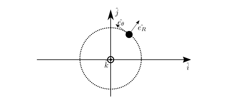
Consider that we have the position vector $\bf\vec{r}$ of a particle, moving in a circular path indicated in the figure below by a dashed line. This vector $\bf\vec{r(t)}$ is described in a fixed reference frame as:
\begin{equation} {\bf\vec{r}}(t) = x(t){\bf\hat{i}} + y(t){\bf\hat{j}} + z(t){\bf\hat{k}} \label{eq_1} \end{equation}

Naturally, we could describe all the kinematic variables in the fixed reference frame. But in circular motions, is convenient to define a basis with a vector in the direction of the position vector $\bf\vec{r}$. So, the vector $\bf\hat{e_R}$ is defined as:
\begin{equation} {\bf\hat{e_R}} = \frac{\bf\vec{r}}{\Vert{\bf\vec{r} }\Vert} \label{eq_2} \end{equation}The second vector of the basis can be obtained by the cross multiplication between $\bf\hat{k}$ and $\bf\hat{e_R}$:
The third vector of the basis is the conventional ${\bf\hat{k}}$ vector.
This basis can be used also for non-circular movements. For a 3D movement, the versor ${\bf\hat{e_R}}$ is obtained by removing the projection of the vector ${\bf\vec{r}}$ onto the versor ${\bf\hat{k}}$:
\begin{equation} {\bf\hat{e_R}} = \frac{\bf\vec{r} - ({\bf\vec{r}.{\bf\hat{k}}){\bf\hat{k}}}}{\Vert\bf\vec{r} - ({\bf\vec{r}.{\bf\hat{k}}){\bf\hat{k}}\Vert}} \label{eq_4} \end{equation}

Note that if the movement is on a plane, the expression above is equal to ${\bf\hat{e_R}} = \frac{\bf\vec{r}}{\Vert{\bf\vec{r} }\Vert}$ since the projection of $\bf\vec{r}$ on the $\bf\hat{k}$ versor is zero.
Time-derivative of the versors ${\bf\hat{e_R}}$ and ${\bf\hat{e_\theta}}$
To obtain the expressions of the velocity and acceleration vectors, it is necessary to obtain the expressions of the time-derivative of the vectors ${\bf\hat{e_R}}$ and ${\bf\hat{e_\theta}}$.
This can be done by noting that:
\begin{align} {\bf\hat{e_R}} &= \cos(\theta){\bf\hat{i}} + \sin(\theta){\bf\hat{j}}\\ {\bf\hat{e_\theta}} &= -\sin(\theta){\bf\hat{i}} + \cos(\theta){\bf\hat{j}} \label{eq_5} \end{align}
Deriving ${\bf\hat{e_R}}$ we obtain:
\begin{equation} \frac{d{\bf\hat{e_R}}}{dt} = -\sin(\theta)\dot\theta{\bf\hat{i}} + \cos(\theta)\dot\theta{\bf\hat{j}} = \dot{\theta}{\bf\hat{e_\theta}} \label{eq_6} \end{equation}
Similarly, we obtain the time-derivative of ${\bf\hat{e_\theta}}$:
\begin{equation} \frac{d{\bf\hat{e_\theta}}}{dt} = -\cos(\theta)\dot\theta{\bf\hat{i}} - \sin(\theta)\dot\theta{\bf\hat{j}} = -\dot{\theta}{\bf\hat{e_R}} \label{eq_7} \end{equation}
Position, velocity and acceleration
Position
The position vector $\bf\vec{r}$, from the definition of $\bf\hat{e_R}$, is:
\begin{equation} {\bf\vec{r}} = R{\bf\hat{e_R}} + z{\bf\hat{k}} \label{eq_8} \end{equation}
where $R = \Vert\bf\vec{r} - ({\bf\vec{r}.{\bf\hat{k}}){\bf\hat{k}}\Vert}$.
Velocity
The velocity vector $\bf\vec{v}$ is obtained by deriving the vector $\bf\vec{r}$:
\begin{equation} {\bf\vec{v}} = \frac{d(R{\bf\hat{e_R}})}{dt} + \dot{z}{\bf\hat{k}} = \dot{R}{\bf\hat{e_R}}+R\frac{d\bf\hat{e_R}}{dt}=\dot{R}{\bf\hat{e_R}}+R\dot{\theta}{\bf\hat{e_\theta}}+ \dot{z}{\bf\hat{k}} \label{eq_9} \end{equation}
Acceleration
The acceleration vector $\bf\vec{a}$ is obtained by deriving the velocity vector:
\begin{align} {\bf\vec{a}} =& \frac{d(\dot{R}{\bf\hat{e_R}}+R\dot{\theta}{\bf\hat{e_\theta}}+\dot{z}{\bf\hat{k}})}{dt}=\\\nonumber =&\ddot{R}{\bf\hat{e_R}}+\dot{R}\frac{d\bf\hat{e_R}}{dt} + \dot{R}\dot{\theta}{\bf\hat{e_\theta}} + R\ddot{\theta}{\bf\hat{e_\theta}} + R\dot{\theta}\frac{d{\bf\hat{e_\theta}}}{dt} + \ddot{z}{\bf\hat{k}}=\\\nonumber =&\ddot{R}{\bf\hat{e_R}}+\dot{R}\dot{\theta}{\bf\hat{e_\theta}} + \dot{R}\dot{\theta}{\bf\hat{e_\theta}} + R\ddot{\theta}{\bf\hat{e_\theta}} - R\dot{\theta}^2{\bf\hat{e_R}}+ \ddot{z}{\bf\hat{k}} =\\ =&\ddot{R}{\bf\hat{e_R}}+2\dot{R}\dot{\theta}{\bf\hat{e_\theta}}+ R\ddot{\theta}{\bf\hat{e_\theta}} - {R}\dot{\theta}^2{\bf\hat{e_R}}+ \ddot{z}{\bf\hat{k}} =\\\nonumber =&(\ddot{R}-R\dot{\theta}^2){\bf\hat{e_R}}+(2\dot{R}\dot{\theta} + R\ddot{\theta}){\bf\hat{e_\theta}}+ \ddot{z}{\bf\hat{k}}\nonumber \label{eq_10} \end{align}
The term $\ddot{R}$ is an acceleration in the radial direction.
The term $R\ddot{\theta}$ is an angular acceleration.
The term $\ddot{z}$ is an acceleration in the $\bf\hat{k}$ direction.
The term $-R\dot{\theta}^2$ is the well known centripetal acceleration.
The term $2\dot{R}\dot{\theta}$ is known as Coriolis acceleration. This term may be difficult to understand intuitively. It appears when there is displacement in the radial and angular directions at the same time.
Important to note
The reader must bear in mind that the use of a different basis to represent the position, velocity or acceleration vectors is only a different representation of the same vector. For example, for the acceleration vector:
\begin{equation} {\bf\vec{a}} = \ddot{x}{\bf\hat{i}}+ \ddot{y}{\bf\hat{j}} + \ddot{z}{\bf\hat{k}}=(\ddot{R}-R\dot{\theta}^2){\bf\hat{e_R}}+(2\dot{R}\dot{\theta} + R\ddot{\theta}){\bf\hat{e_\theta}} + \ddot{z}{\bf\hat{k}}=\dot{\Vert\bf\vec{v}\Vert}{\bf\hat{e}_t}+\frac{{\Vert\bf\vec{v}\Vert}^2}{\rho}{\bf\hat{e}_n} \label{eq_11} \end{equation}
In which the last equality is the acceleration vector represented in the path-coordinate of the particle (see http://nbviewer.jupyter.org/github/BMClab/bmc/blob/master/notebooks/Time-varying%20frames.ipynb).
Example
Consider a particle following the spiral path described below:
\begin{equation} {\bf\vec{r}}(t) = \left(2\sqrt{t}\cos(t)\right){\bf\hat{i}}+ \left(2\sqrt{t}\sin(t)\right){\bf\hat{j}} \label{eq_12} \end{equation}
Solving numerically
t = np.linspace(0.01,10,30).reshape(-1,1) #create a time vector and reshapes it to a column vector
R = 2*np.sqrt(t)
theta = t
rx = R*np.cos(theta)
ry = R*np.sin(theta)
r = np.hstack((rx, ry)) # creates the position vector by stacking rx and ry horizontally
e_r = r/np.linalg.norm(r, axis=1, keepdims=True) # defines e_r vector
e_theta = np.cross([0,0,1],e_r)[:,0:-1] # defines e_theta vector
dt = t[1,0] #defines delta_t
Rdot = np.gradient(R, dt, axis=0) #find the R derivative
thetaDot = np.gradient(theta, dt, axis=0) #find the angle derivative
v = Rdot*e_r +R*thetaDot*e_theta # find the linear velocity.
Rddot = np.gradient(Rdot, dt, axis=0)
thetaddot = np.gradient(thetaDot, dt, axis=0)
a = ((Rddot - R*thetaDot**2)*e_r
     + (2*Rdot*thetaDot + R*thetaddot)*e_theta)
The versors $\bf\hat{e_R}$, $\bf\hat{e_\theta}$ are plotted below at some points of the path.
from matplotlib.patches import FancyArrowPatch
%matplotlib inline
plt.rcParams['figure.figsize'] = (8,8)
fig = plt.figure()

ax = fig.add_axes([0,0,1,1])
plt.plot(r[:,0],r[:,1],'.')
for i in np.arange(len(t)-2):
    vec1 = FancyArrowPatch(r[i,:],r[i,:]+e_r[i,:],mutation_scale=30,color='r', label='e_r')
    vec2 = FancyArrowPatch(r[i,:],r[i,:]+e_theta[i,:],mutation_scale=30,color='g', label='e_theta')
    ax.add_artist(vec1)
    ax.add_artist(vec2)
plt.xlim((-10,10))
plt.ylim((-10,10))
plt.grid()
plt.legend([vec1, vec2],[r'$\vec{e_r}$', r'$\vec{e_{\theta}}$'])
plt.show()

The velocity and acceleleration of the particle are plotted below at some points of the path.
from matplotlib.patches import FancyArrowPatch
%matplotlib inline
plt.rcParams['figure.figsize'] = (8,8)
fig = plt.figure()
plt.plot(r[:,0],r[:,1],'.')
ax = fig.add_axes([0,0,1,1])
for i in np.arange(len(t)-2):
    vec1 = FancyArrowPatch(r[i,:],r[i,:]+v[i,:],mutation_scale=10,color='r')
    vec2 = FancyArrowPatch(r[i,:],r[i,:]+a[i,:],mutation_scale=10,color='g')
    ax.add_artist(vec1)
    ax.add_artist(vec2)
plt.xlim((-10,10))
plt.ylim((-10,10))
plt.grid()
plt.legend([vec1, vec2],[r'$\vec{v}$', r'$\vec{a}$'])
plt.show()

Solved symbolically (extra reading)
O = sym.vector.CoordSys3D(' ')
t = sym.symbols('t')
r = 2*sym.sqrt(t)*sym.cos(t)*O.i+2*sym.sqrt(t)*sym.sin(t)*O.j
r
plot_parametric(r.dot(O.i),r.dot(O.j),(t,0,10))

<sympy.plotting.plot.Plot at 0x7fa6826b1c10>
e_r = sym.simplify(r/sym.sqrt(r.dot(O.i)**2+r.dot(O.j)**2+r.dot(O.k)**2))
e_r
e_theta = O.k.cross(e_r)
e_theta
from matplotlib.patches import FancyArrowPatch
plt.rcParams['figure.figsize'] = (8,8)
fig = plt.figure()
ax = fig.add_axes([0, 0, 1, 1])
ax.axis("on")
time = np.linspace(0,10,30)
for instant in time:
    vt = FancyArrowPatch([float(r.dot(O.i).subs(t,instant)),float(r.dot(O.j).subs(t,instant))],
                         [float(r.dot(O.i).subs(t,instant))+float(e_r.dot(O.i).subs(t,instant)),
                          float(r.dot(O.j).subs(t, instant))+float(e_r.dot(O.j).subs(t,instant))],
                         mutation_scale=20,
                         arrowstyle="->",color="r",label='${{e_r}}$')
    vn = FancyArrowPatch([float(r.dot(O.i).subs(t, instant)),float(r.dot(O.j).subs(t,instant))],
                         [float(r.dot(O.i).subs(t, instant))+float(e_theta.dot(O.i).subs(t, instant)),
                          float(r.dot(O.j).subs(t, instant))+float(e_theta.dot(O.j).subs(t, instant))],
                         mutation_scale=20,
                         arrowstyle="->",color="g",label='${{e_{theta}}}$')
    ax.add_artist(vn)
    ax.add_artist(vt)
plt.xlim((-10,10))
plt.ylim((-10,10))
plt.legend(handles=[vt,vn],fontsize=20)
plt.grid()
plt.show()

R = 2*sym.sqrt(t)
Rdot = sym.diff(R,t)
Rddot = sym.diff(Rdot,t)
theta = t
thetadot = sym.diff(theta, t)
thetaddot = sym.diff(thetadot, t)
thetaddot
v = Rdot*e_r + R*thetadot*e_theta
v
a = (Rddot - R*thetadot**2)*e_r + (2*Rdot*thetadot+R*thetaddot)*e_theta
aCor = 2*Rdot*thetadot*e_theta
aCor
a
from matplotlib.patches import FancyArrowPatch
plt.rcParams['figure.figsize'] = (8,8)
fig = plt.figure()
ax = fig.add_axes([0, 0, 1, 1])
ax.axis("on")
time = np.linspace(0.1,10,30)
for instant in time:
    vt = FancyArrowPatch([float(r.dot(O.i).subs(t,instant)),float(r.dot(O.j).subs(t,instant))],
                         [float(r.dot(O.i).subs(t,instant))+float(v.dot(O.i).subs(t,instant)),
                          float(r.dot(O.j).subs(t, instant))+float(v.dot(O.j).subs(t,instant))],
                         mutation_scale=20,
                         arrowstyle="->",color="r",label='${{v}}$')
    vn = FancyArrowPatch([float(r.dot(O.i).subs(t, instant)),float(r.dot(O.j).subs(t,instant))],
                         [float(r.dot(O.i).subs(t, instant))+float(a.dot(O.i).subs(t, instant)),
                          float(r.dot(O.j).subs(t, instant))+float(a.dot(O.j).subs(t, instant))],
                         mutation_scale=20,
                         arrowstyle="->",color="g",label='${{a}}$')
    vc = FancyArrowPatch([float(r.dot(O.i).subs(t, instant)),float(r.dot(O.j).subs(t,instant))],
                         [float(r.dot(O.i).subs(t, instant))+float(aCor.dot(O.i).subs(t, instant)),
                          float(r.dot(O.j).subs(t, instant))+float(aCor.dot(O.j).subs(t, instant))],
                         mutation_scale=20,
                         arrowstyle="->",color="b",label='${{a_{Cor}}}$')
    ax.add_artist(vn)
    ax.add_artist(vt)
    ax.add_artist(vc)
plt.xlim((-10,10))
plt.ylim((-10,10))
plt.legend(handles=[vt,vn,vc],fontsize=20)
plt.grid()
plt.show()

Further reading
- Read pages 916-931 of the 18th chapter of the [Ruina and Rudra's book] (http://ruina.tam.cornell.edu/Book/index.html) about polar coordinates.
Video lectures on the Internet
- Khan Academy:
Problems
- Find the polar basis (using the computer) for a projectile motion of a particle following the parametric equation below:
- Problems from 15.1.1 to 15.1.14 from Ruina and Rudra's book,
- Problems from 18.1.1 to 18.1.8 and 18.1.10 from Ruina and Rudra's book.
- Solve the problems 1.19 and 1.20 from Rade's book.
Reference
- Ruina A, Rudra P (2019) Introduction to Statics and Dynamics. Oxford University Press.