# HIDDEN

from datascience import *
import numpy as np

%matplotlib inline
import matplotlib.pyplot as plots
plots.style.use('fivethirtyeight')
import math
Inspired by Peter Norvig's A Concrete Introduction to Probability
Probability is the study of the observations that are generated by sampling from a known distribution. The statistical methods we have studied so far allow us to reason about the world from data. Probability allows us to reason in the opposite directions: what observations result from know facts about the world.
In practice, we rarely know precisely how random processes in the world work. Even the simplest random process such as flipping a coin is not as simple as one might assume. Nonetheless, our ability to reason about what data will result from a known random process is useful in many aspects of data science. Fundamentally, the rules of probability allow us to reason about the consequences of assumptions we make.
Probability Distributions
Probability uses the following vocabulary to describe the relationship between known distributions and their observed outcomes.
- Experiment: An occurrence with an uncertain outcome that we can observe. For example, the result of rolling two dice in sequence.
- Outcome: The result of an experiment; one particular state of the world. For example: the first die comes up 4 and the second comes up 2. This outcome could be summarized as
(4, 2). - Sample Space: The set of all possible outcomes for the experiment. For example,
{(1, 1), (1, 2), (1, 3), ..., (1, 6), (2, 1), (2, 2), ... (6, 4), (6, 5), (6, 6)}are all possible outcomes of rolling two dice in sequence. There are6 * 6 = 36different outcomes. - Event: A subset of possible outcomes that together have some property we are interested in. For example, the event "the two dice sum to 5" is the set of outcomes {(1, 4), (2, 3), (3, 2), (4, 1)}.
- Probability: The proportion of experiments for which the event occurs. For example, the probability that the two dice sum to 5 is
4/36or1/9. - Distribution: The probability of all events.
The important part of this terminology is that the sample space is the set of all outcomes, and an event is a subset of the sample space. For an outcome that is an element of an event, we say that it is an outcome for which that event occurs.
Multinomial Distributions
There are many kinds of distributions, but we will focus on the case where the sample space is a fixed, finite set of mutually exclusive outcomes, called a multinomial distribution.
For example, either the two dice come up (2, 1) or they come up (4, 5) in a single roll (but both cannot occur), and there are exactly 36 outcome possibilities that each occur with equal chance.
two_dice = Table(['First', 'Second', 'Chance'])
for first in np.arange(1, 7):
    for second in np.arange(1, 7):
        two_dice.append([first, second, 1/36])
two_dice.set_format('Chance', PercentFormatter(1))
| First | Second | Chance |
|---|---|---|
| 1 | 1 | 2.8% |
| 1 | 2 | 2.8% |
| 1 | 3 | 2.8% |
| 1 | 4 | 2.8% |
| 1 | 5 | 2.8% |
| 1 | 6 | 2.8% |
| 2 | 1 | 2.8% |
| 2 | 2 | 2.8% |
| 2 | 3 | 2.8% |
| 2 | 4 | 2.8% |
... (26 rows omitted)
The outcomes are not always equally likely. In the example of two dice rolled in sequence, there are 36 different outcomes that each have a 1/36 chance of occurring. If two dice are rolled together and only the sum of the result is observed, instead there are 11 outcomes that have various different chances.
two_dice_sums = Table(['Sum', 'Chance']).with_rows([
        [ 2, 1/36], [ 3, 2/36], [ 4, 3/36], [5, 4/36], [6, 5/36], [7, 6/36],
        [12, 1/36], [11, 2/36], [10, 3/36], [9, 4/36], [8, 5/36],
    ]).sort(0)
two_dice_sums.set_format('Chance', PercentFormatter(1))
| Sum | Chance |
|---|---|
| 2 | 2.8% |
| 3 | 5.6% |
| 4 | 8.3% |
| 5 | 11.1% |
| 6 | 13.9% |
| 7 | 16.7% |
| 8 | 13.9% |
| 9 | 11.1% |
| 10 | 8.3% |
| 11 | 5.6% |
... (1 rows omitted)
Outcomes and Events
These two different dice distributions are closely related to each other. Let's see how.
In a multinomial distribution, each outcome alone is an event with its own chance (or probability). The chances of all outcomes sum to 1. The probability of any event is the sum of the probabilities of the outcomes in that event. Therefore, by writing down the chance of each outcome, we implicitly describe the probability of every event for the whole distribution.
Let's consider the event that the sum of the dice in two sequential rolls is 5. We can represent that event as the matching rows in the two_dice table.
dice_sums = two_dice.column('First') + two_dice.column('Second')
sum_of_5 = two_dice.where(dice_sums == 5)
sum_of_5
| First | Second | Chance |
|---|---|---|
| 1 | 4 | 2.8% |
| 2 | 3 | 2.8% |
| 3 | 2 | 2.8% |
| 4 | 1 | 2.8% |
The probability of the event is the sum of the resulting chances.
sum(sum_of_5.column('Chance'))
0.1111111111111111
If we consistently store the probabilities of individual outcomes in a column called Chance, then we can define the probability of any event using the P function.
def P(event):
    return sum(event.column('Chance'))

P(sum_of_5)
0.1111111111111111
One distribution's events can be another distribution's outcomes, as is the case with the two_dice and two_dice_sum distributions. There are 11 different possible sums in the two_dice table, and these are 11 different mutually exclusive events.
with_sums = two_dice.with_column('Sum', dice_sums)
with_sums
| First | Second | Chance | Sum |
|---|---|---|---|
| 1 | 1 | 2.8% | 2 |
| 1 | 2 | 2.8% | 3 |
| 1 | 3 | 2.8% | 4 |
| 1 | 4 | 2.8% | 5 |
| 1 | 5 | 2.8% | 6 |
| 1 | 6 | 2.8% | 7 |
| 2 | 1 | 2.8% | 3 |
| 2 | 2 | 2.8% | 4 |
| 2 | 3 | 2.8% | 5 |
| 2 | 4 | 2.8% | 6 |
... (26 rows omitted)
Grouping these outcomes by their sum shows how many different outcomes appear in each event.
with_sums.group('Sum')
| Sum | count |
|---|---|
| 2 | 1 |
| 3 | 2 |
| 4 | 3 |
| 5 | 4 |
| 6 | 5 |
| 7 | 6 |
| 8 | 5 |
| 9 | 4 |
| 10 | 3 |
| 11 | 2 |
... (1 rows omitted)
Finally, the chance of each sum event is the total chance of all outcomes that match the sum event. In this way, we can generate the two_dice_sums distribution via addition.
grouped = with_sums.select(['Sum', 'Chance']).group('Sum', sum)
grouped.relabeled(1, 'Chance').set_format('Chance', PercentFormatter(1))
| Sum | Chance |
|---|---|
| 2 | 2.8% |
| 3 | 5.6% |
| 4 | 8.3% |
| 5 | 11.1% |
| 6 | 13.9% |
| 7 | 16.7% |
| 8 | 13.9% |
| 9 | 11.1% |
| 10 | 8.3% |
| 11 | 5.6% |
... (1 rows omitted)
Both distributions will assign the same probability to certain events. For example, the probability of the event that the sum of the dice is above 8 can be computed from either distribution.
P(with_sums.where('Sum', 8))
0.1388888888888889
P(two_dice_sums.where('Sum', 8))
0.1388888888888889
U.S. Birth Times
Here's an example based on data collected in the world.
More babies in the United States are born in the morning than the night. In 2013, the Center for Disease Control measured the following proportions of babies for each hour of the day. The Time column is a description of each hour, and the Hour column is its numeric equivalent.
birth = Table.read_table('birth_time.csv').select(['Time', 'Hour', 'Chance'])
birth.set_format('Chance', PercentFormatter(1)).show()
| Time | Hour | Chance |
|---|---|---|
| 6 a.m. | 6 | 2.9% |
| 7 a.m. | 7 | 4.5% |
| 8 a.m. | 8 | 6.3% |
| 9 a.m. | 9 | 5.0% |
| 10 a.m. | 10 | 5.0% |
| 11 a.m. | 11 | 5.0% |
| Noon | 12 | 6.0% |
| 1 p.m. | 13 | 5.7% |
| 2 p.m. | 14 | 5.1% |
| 3 p.m. | 15 | 4.8% |
| 4 p.m. | 16 | 4.9% |
| 5 p.m. | 17 | 5.0% |
| 6 p.m. | 18 | 4.5% |
| 7 p.m. | 19 | 4.0% |
| 8 p.m. | 20 | 4.0% |
| 9 p.m. | 21 | 3.7% |
| 10 p.m. | 22 | 3.5% |
| 11 p.m. | 23 | 3.3% |
| Midnight | 0 | 2.9% |
| 1 a.m. | 1 | 2.9% |
| 2 a.m. | 2 | 2.8% |
| 3 a.m. | 3 | 2.7% |
| 4 a.m. | 4 | 2.7% |
| 5 a.m. | 5 | 2.8% |
If we assume that this distribution describes the world correctly, what is the chance that a baby will be born between 8 a.m. and 6 p.m.? It turns out that more than half of all babies are born during "business hours", even though this time interval only covers 5/12 of the day.
business_hours = birth.where('Hour', are.between(8, 18))
business_hours
| Time | Hour | Chance |
|---|---|---|
| 8 a.m. | 8 | 6.3% |
| 9 a.m. | 9 | 5.0% |
| 10 a.m. | 10 | 5.0% |
| 11 a.m. | 11 | 5.0% |
| Noon | 12 | 6.0% |
| 1 p.m. | 13 | 5.7% |
| 2 p.m. | 14 | 5.1% |
| 3 p.m. | 15 | 4.8% |
| 4 p.m. | 16 | 4.9% |
| 5 p.m. | 17 | 5.0% |
P(business_hours)
0.52800000000000002
On the other hand, births late at night are uncommon. The chance of having a baby between midnight and 6 a.m. is much less than 25%, even though this time interval covers 1/4 of the day.
P(birth.where('Hour', are.between(0, 6)))
0.16799999999999998
Conditional Distributions
A common way to transform one distribution into another is to condition on an event. Conditioning means assuming that the event occurs. The conditional distribution given an event takes the chances of all outcomes for which the event occurs and scales up their chances so that they sum to 1.
To scale up the chances, we divide the chance of each outcome in the event by the probability of the event. For example, if we condition on the event that the sum of two dice is above 8, we arrive at the following conditional distribution.
above_8 = two_dice_sums.where('Sum', are.above(8))
given_8 = above_8.with_column('Chance', above_8.column('Chance') / P(above_8))
given_8
| Sum | Chance |
|---|---|
| 9 | 40.0% |
| 10 | 30.0% |
| 11 | 20.0% |
| 12 | 10.0% |
A conditional distribution describes the chances under the original distribution, updated to reflect a new piece of information. In this case, we see the chances under the original two_dice_sums distribution, given that the sum is above 8.
The conditioning operation can be expressed by the given function, which takes an event table and returns the corresponding conditional distributon.
def given(event):
    return event.with_column('Chance', event.column('Chance') / P(event))

given(two_dice_sums.where('Sum', are.above(8)))
| Sum | Chance |
|---|---|
| 9 | 40.0% |
| 10 | 30.0% |
| 11 | 20.0% |
| 12 | 10.0% |
Given that a baby is born in the US during business hours (between 8 a.m. and 6 p.m.), what are the chances that it is born before noon? To answer this question, we first form the conditional distribution given business hours, then compute the probability of the event that the baby is born before noon.
given(business_hours)
| Time | Hour | Chance |
|---|---|---|
| 8 a.m. | 8 | 11.9% |
| 9 a.m. | 9 | 9.5% |
| 10 a.m. | 10 | 9.5% |
| 11 a.m. | 11 | 9.5% |
| Noon | 12 | 11.4% |
| 1 p.m. | 13 | 10.8% |
| 2 p.m. | 14 | 9.7% |
| 3 p.m. | 15 | 9.1% |
| 4 p.m. | 16 | 9.3% |
| 5 p.m. | 17 | 9.5% |
P(given(business_hours).where('Hour', are.below(12)))
0.40340909090909094
This result is not the same as the chance that a baby is born between 8 a.m. and noon in general.
morning = birth.where('Hour', are.between(8, 12))
P(morning)
0.21300000000000002
Nor is it the chance that a baby is born before noon in general.
P(birth.where('Hour', are.below(12)))
0.45500000000000007
Instead, it is the probability that both the event and the conditioning event are true (i.e., that the birth is in the morning), divided by the probability of the conditioning event (i.e., that the birth is during business hours).
P(morning) / P(business_hours)
0.40340909090909094
The morning event is a joint event that can be described as both during business hours and before noon. A joint event is just an event, but one that is described by the intersection of two other events.
business_hours.where('Hour', are.below(12))
| Time | Hour | Chance |
|---|---|---|
| 8 a.m. | 8 | 6.3% |
| 9 a.m. | 9 | 5.0% |
| 10 a.m. | 10 | 5.0% |
| 11 a.m. | 11 | 5.0% |
In general, the probability of an event B (e.g., before noon) conditioned on an event A (e.g., during business hours) is the probability of the joint event of A and B divided by the probability of the conditioning event A.
P(business_hours.where('Hour', are.below(12))) / P(business_hours)
0.40340909090909094
The standard notation for this relationship uses a vertical bar for conditioning and a comma for a joint event.
$$P(B | A) = \frac{P(A, B)}{P(A)}$$Joint Distributions
A joint event is one in which two different events both occur. Similarly, a joint outcome is an outcome that is composed of two different outcomes. For example, the outcomes of the two_dice distribution are each joint outcomes of the first and second dice rolls.
two_dice
| First | Second | Chance |
|---|---|---|
| 1 | 1 | 2.8% |
| 1 | 2 | 2.8% |
| 1 | 3 | 2.8% |
| 1 | 4 | 2.8% |
| 1 | 5 | 2.8% |
| 1 | 6 | 2.8% |
| 2 | 1 | 2.8% |
| 2 | 2 | 2.8% |
| 2 | 3 | 2.8% |
| 2 | 4 | 2.8% |
... (26 rows omitted)
Another common way to transform distributions is to form a joint distribution from conditional distributions. The definition of a conditional probability provides a formula for computing a joint probability, simply by multiplying both sides of the equation above by $P(B)$.
$$ P(B|A) \times P(A) = P(A, B) $$The chance of each outcome of a joint distribution can be computed from the probability of the first outcome and the conditional probability of the second outcome given the first outcome. In the two_dice table above, the chance of any first outcome is 1/6, and the chance of any second outcome given any first outcome is 1/6, so the chance of any joint outcome is 1/36 or 2.8%.
U.S. Birth Days
The CDC also published that in 2013, 78.25% of babies born on weekdays (Monday through Friday) and 21.75% of babies were born on weekends (Saturday and Sunday). Notably, this distribution is not 5/7 (71.4%) to 2/7 (28.6%), but instead favors weekdays.
Moreover, the CDC published the conditional distributions of 2013 birth times, given a weekday birth (green) and given a weekend birth (gray). The black line is the distribution of all births.
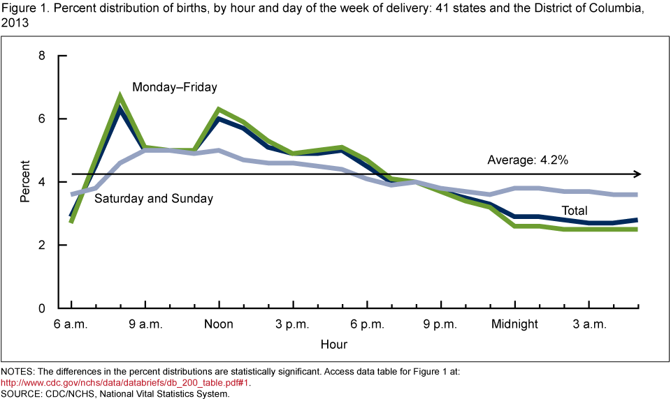
All of the proportions used to generate this chart appear in the birth_day table.
birth_day = Table.read_table('birth_time.csv').drop('Chance')
birth_day.set_format([2, 3], PercentFormatter(1))
| Time | Hour | Weekday | Weekend |
|---|---|---|---|
| 6 a.m. | 6 | 2.7% | 3.6% |
| 7 a.m. | 7 | 4.7% | 3.8% |
| 8 a.m. | 8 | 6.7% | 4.6% |
| 9 a.m. | 9 | 5.1% | 5.0% |
| 10 a.m. | 10 | 5.0% | 5.0% |
| 11 a.m. | 11 | 5.0% | 4.9% |
| Noon | 12 | 6.3% | 5.0% |
| 1 p.m. | 13 | 5.9% | 4.7% |
| 2 p.m. | 14 | 5.3% | 4.6% |
| 3 p.m. | 15 | 4.9% | 4.6% |
... (14 rows omitted)
The Weekday and Weekend columns are the chances of two different conditional distributions.
weekday = birth_day.select(['Hour', 'Weekday']).relabeled(1, 'Chance')
weekend = birth_day.select(['Hour', 'Weekend']).relabeled(1, 'Chance')
The joint distribution is created by multiplying each conditional chance column by the corresponding probability of the conditioning event. In this case, we multiply weekday chances by the chance that the baby was born on a weekday (78.25%); likewise, we multiply weekend chances by the chance that the baby was born on a weekend (21.75%).
birth_joint = Table(['Day', 'Hour', 'Chance'])
for row in weekday.rows:
    birth_joint.append(['Weekday', row.item('Hour'), row.item('Chance') * 0.7825])
for row in weekend.rows:
    birth_joint.append(['Weekend', row.item('Hour'), row.item('Chance') * 0.2175])
birth_joint.set_format('Chance', PercentFormatter(1))
| Day | Hour | Chance |
|---|---|---|
| Weekday | 6 | 2.1% |
| Weekday | 7 | 3.7% |
| Weekday | 8 | 5.2% |
| Weekday | 9 | 4.0% |
| Weekday | 10 | 3.9% |
| Weekday | 11 | 3.9% |
| Weekday | 12 | 4.9% |
| Weekday | 13 | 4.6% |
| Weekday | 14 | 4.1% |
| Weekday | 15 | 3.8% |
... (38 rows omitted)
This joint distribution has 48 joint outcomes, and the total chance sums to 1.
P(birth_joint)
1.0
Now, we can compute the probability of any event that involves days and hours. For example, the chance of a weekday morning birth is quite high.
P(birth_joint.where('Day', 'Weekday').where('Hour', are.between(8, 12)))
0.17058499999999999
We have seen that less than 22% of babies are born on weekends. However, if we know that a baby was born between 5 a.m. and 6 a.m., then the chances that it is a weekend baby are quite a bit higher than 22%.
early_morning = birth_joint.where('Hour', 5)
early_morning
| Day | Hour | Chance |
|---|---|---|
| Weekday | 5 | 2.0% |
| Weekend | 5 | 0.8% |
P(given(early_morning).where('Day', 'Weekend'))
0.28584466551063248
Bayes' Rule
In the final example above, we began with a distribution over weekday and weekend births, $P(A)$, along with conditional distributions over hours, $P(B|A)$. We were able to compute the probability of a weekend birth conditioned on an hour, an outcome in the distribution $P(A|B)$. Bayes' rule is the formula that expresses the relationship between all of these quantities.
$$ P(A|B) = \frac{P(A) \times P(B|A)}{P(B)} $$The numerator on the right-hand side is just the joint probability of A and B. Bayes' rule writes this probability in its expanded form because so often we are given these two components and must form the joint distribution through multiplication.
The denominator on the right-hand side is an event that can be computed from the joint probability. For example, the early_morning event in the example above is an event just about hours, but it includes all joint outcomes where the correct hour occurs.
Each probability in this equation has a name. The names are derived from the most typical application of Bayes' rule, which is to update one's beliefs based on new evidence.
- $P(A)$ is called the prior; it is the probability of event A before any evidence is observed.
- $P(B|A)$ is called the likelihood; it is the conditional probability of the evidence event B given the event A.
- $P(B)$ is called the evidence; it is the probability of the evidence event B for any outcome.
- $P(A|B)$ is called the posterior; it is the probabilyt of event A after evidence event B is observed.
Depending on the joint distribution of A and B, observing some B can make A more or less likely.
Diagnostic Example
In a population, there is a rare disease. Researchers have developed a medical test for the disease. Mostly, the test correctly identifies whether or not the tested person has the disease. But sometimes, the test is wrong. Here are the relevant proportions.
- 1% of the population has the disease
- If a person has the disease, the test returns the correct result with chance 99%.
- If a person does not have the disease, the test returns the correct result with chance 99.5%.
One person is picked at random from the population. Given that the person tests positive, what is the chance that the person has the disease?
We begin by partitioning the population into four categories in the tree diagram below.

By Bayes' Rule, the chance that the person has the disease given that he or she has tested positive is the chance of the top "Test Positive" branch relative to the total chance of the two "Test Positive" branches. The answer is $$ \frac{0.01 \times 0.99}{0.01 \times 0.99 ~+~ 0.99 \times 0.005} ~=~ 0.667 $$
# The person is picked at random from the population.

# By Bayes' Rule:
# Chance that the person has the disease, given that test was +

(0.01*0.99)/(0.01*0.99 + 0.99*0.005)
0.6666666666666666
This is 2/3, and it seems rather small. The test has very high accuracy, 99% or higher. Yet is our answer saying that if a patient gets tested and the test result is positive, there is only a 2/3 chance that he or she has the disease?
To understand our answer, it is important to recall the chance model: our calculation is valid for a person picked at random from the population. Among all the people in the population, the people who test positive split into two groups: those who have the disease and test positive, and those who don't have the disease and test positive. The latter group is called the group of false positives. The proportion of true positives is twice as high as that of the false positives – $0.01 \times 0.99$ compared to $0.99 \times 0.005$ – and hence the chance of a true positive given a positive test result is $2/3$. The chance is affected both by the accuracy of the test and also by the probability that the sampled person has the disease.
The same result can be computed using a table. Below, we begin with the joint distribution over true health and test results.
rare = Table(['Health', 'Test', 'Chance']).with_rows([
        ['Diseased', 'Positive', 0.01 * 0.99],
        ['Diseased', 'Negative', 0.01 * 0.01],
        ['Not Diseased', 'Positive', 0.99 * 0.005],
        ['Not Diseased', 'Negative', 0.99 * 0.995]
    ])
rare
| Health | Test | Chance |
|---|---|---|
| Diseased | Positive | 0.0099 |
| Diseased | Negative | 0.0001 |
| Not Diseased | Positive | 0.00495 |
| Not Diseased | Negative | 0.98505 |
The chance that a person selected at random is diseased, given that they tested positive, is computed from the following expression.
positive = rare.where('Test', 'Positive')
P(given(positive).where('Health', 'Diseased'))
0.66666666666666663
But a patient who goes to get tested for a disease is not well modeled as a random member of the population. People get tested because they think they might have the disease, or because their doctor thinks so. In such a case, saying that their chance of having the disease is 1% is not justified; they are not picked at random from the population.
So, while our answer is correct for a random member of the population, it does not answer the question for a person who has walked into a doctor's office to be tested.
To answer the question for such a person, we must first ask ourselves what is the probability that the person has the disease. It is natural to think that it is larger than 1%, as the person has some reason to believe that he or she might have the disease. But how much larger?
This cannot be decided based on relative frequencies. The probability that a particular individual has the disease has to be based on a subjective opinion, and is therefore called a subjective probability. Some researchers insist that all probabilities must be relative frequencies, but subjective probabilities abound. The chance that a candidate wins the next election, the chance that a big earthquake will hit the Bay Area in the next decade, the chance that a particular country wins the next soccer World Cup: none of these are based on relative frequencies or long run frequencies. Each one contains a subjective element.
It is fine to work with subjective probabilities as long as you keep in mind that there will be a subjective element in your answer. Be aware also that different people can have different subjective probabilities of the same event. For example, the patient's subjective probability that he or she has the disease could be quite different from the doctor's subjective probability of the same event. Here we will work from the patient's point of view.
Suppose the patient assigned a number to his/her degree of uncertainty about whether he/she had the disease, before seeing the test result. This number is the patient's subjective prior probability of having the disease.
If that probability were 10%, then the probabilities on the left side of the tree diagram would change accordingly, with the 0.1 and 0.9 now interpreted as subjective probabilities:

The change has a noticeable effect on the answer, as you can see by running the cell below.
# Subjective prior probability of 10% that the person has the disease

# By Bayes' Rule:
# Chance that the person has the disease, given that test was +

(0.1*0.99)/(0.1*0.99 + 0.9*0.005)
0.9565217391304347
If the patient's prior probability of having the disease is 10%, then after a positive test result the patient must update that probability to over 95%. This updated probability is called a posterior probability. It is calculated after learning the test result.
If the patient's prior probability of havng the disease is 50%, then the result changes yet again.

# Subjective prior probability of 50% that the person has the disease

# By Bayes' Rule:
# Chance that the person has the disease, given that test was +

(0.5*0.99)/(0.5*0.99 + 0.5*0.005)
0.9949748743718593
Starting out with a 50-50 subjective chance of having the disease, the patient must update that chance to about 99.5% after getting a positive test result.
Computational Note. In the calculation above, the factor of 0.5 is common to all the terms and cancels out. Hence arithmetically it is the same as a calculation where the prior probabilities are apparently missing:
0.99/(0.99 + 0.005)
0.9949748743718593
But in fact, they are not missing. They have just canceled out. When the prior probabilities are not all equal, then they are all visible in the calculation as we have seen earlier.
In machine learning applications such as spam detection, Bayes' Rule is used to update probabilities of messages being spam, based on new messages being labeled Spam or Not Spam. You will need more advanced mathematics to carry out all the calculations. But the fundamental method is the same as what you have seen in this section.