from IPython.core.display import HTML

print("Setting custom CSS for the IPython Notebook")
styles = open('custom.css', 'r').read()
HTML(styles)
Setting custom CSS for the IPython Notebook
import scipy
import numpy as np
import matplotlib
%matplotlib inline
%pylab inline

import matplotlib.pyplot as plt
import seaborn as sns
sns.set_context("talk")
sns.set_style("white")

import pandas as pd

from matplotlib.colors import ListedColormap
import sklearn
import sklearn.decomposition
import sklearn.neighbors
import sklearn.datasets

cmap_light = matplotlib.colors.ListedColormap(['#FFAAAA', '#AAFFAA', '#AAAAFF'])
Populating the interactive namespace from numpy and matplotlib
# generate plots for later

# ML in 10 minutes plot
#cheat to get the same "random" numbers
np.random.seed(seed=99)

# make some data up
mean1 = [3,3]
mean2 = [8,8]
cov = [[1.0,0.0],[0.0,1.0]]

#create some points
x1 = np.random.multivariate_normal(mean1,cov,50)
x2 = np.random.multivariate_normal(mean2,cov,50)

plt.scatter(x1[:,0],x1[:,1], c='r', s=100)
plt.scatter(x2[:,0],x2[:,1], c='b', s=100)

plt.plot([2,10],[10,1], c='g', linewidth=5.0)

plt.title("ML in One Picture")
plt.xlabel("feature 1")
plt.ylabel("feature 2")

fig_ml_in_10 = plt.gcf()

# features matter plot
#cheat to get the same "random" numbers
np.random.seed(seed=99)

# make some data up
mean1 = [6,6]
mean2 = [6,6]
cov = [[1.0,0.0],[0.0,1.0]]

#create some points
x1 = np.random.multivariate_normal(mean1,cov,50)
x2 = np.random.multivariate_normal(mean2,cov,50)

plt.scatter(x1[:,0],x1[:,1], c='r', s=100)
plt.scatter(x2[:,0],x2[:,1], c='b', s=100)

plt.plot([2,10],[10,1], c='g', linewidth=5.0)

plt.title("Apples and Oranges")
plt.xlabel("Roundness")
plt.ylabel("Weight")

fig_features_matter_confused = plt.gcf()

#cheat to get the same "random" numbers
np.random.seed(seed=42)

# make some data up
mean1 = [5,5]
mean2 = [11,5]
cov = [[1.0,0.0],[0.0,1.0]]

#create some points
x1 = np.random.multivariate_normal(mean1,cov,50)
x2 = np.random.multivariate_normal(mean2,cov,50)

plt.scatter(x1[:,0],x1[:,1], c='r', s=100)
plt.scatter(x2[:,0],x2[:,1], c='b', s=100)

plt.plot([8,8],[2,10], c='g', linewidth=5.0)

plt.title("Apples and Oranges")
plt.xlabel("Color")
plt.ylabel("Shape")

fig_features_matter_separated = plt.gcf()

#cheat to get the same "random" numbers
np.random.seed(seed=99)

# make some data up
mean1 = [3,3]
mean2 = [8,8]
cov = [[1.0,0.0],[0.0,1.0]]

#create some points
x1 = np.random.multivariate_normal(mean1,cov,50)
x2 = np.random.multivariate_normal(mean2,cov,50)

plt.scatter(x1[:,0],x1[:,1], c='r', s=100)
plt.scatter(x2[:,0],x2[:,1], c='b', s=100)
plt.scatter([6],[9], c='k', s=200)

plt.plot([2,10],[10,1], c='g', linewidth=5.0)

plt.title("ML in One Picture")
plt.xlabel("feature 1")
plt.ylabel("feature 2")

fig_prediction = plt.gcf()

Introduction to Machine Learning
Analyze training data
Make predictions for new data points
- supervised learning
- data has labels
Find patterns in the data
- unsupervised learning
- data has no labels
Examples for Supervised Learning
- face detection
- handwritten digit recognition
- sound classification for hearing aids
- spam filtering
- recommender systems
Examples for Unsupervised Learning
- dimensionality reduction
- cocktail party problem
- fraud detection
- google image search categories
Somewhere in Between
reinforcement learning
- flappy bird agent
semi-supervised learning
- music classification
Supervised Learning
fig_ml_in_10
Features Matter!
fig_features_matter_confused
Features Matter!
fig_features_matter_separated
Self Driving Car
- *** What features do you need to drive a car? ***
Self Driving Car

Just Measure Everything?
Data volume
Computational overhead
Curse of Dimensionality
Prediction
fig_prediction
# get the data
x = np.concatenate((x1, x2))

# get the labels
ones = np.ones((50,))
y = np.concatenate((ones*0, ones))
K Nearest Neighbors
predict class of new data point by majority vote of K nearest neighbors
very simple
but good performance
K Nearest Neighbors

"train" a KNN Classifier
*** Why is this not really training? ***
k = 1 # number of neighbors

classifier = sklearn.neighbors.KNeighborsClassifier(n_neighbors=k)
classifier.fit(x,y)
KNeighborsClassifier(algorithm='auto', leaf_size=30, metric='minkowski',
           n_neighbors=1, p=2, weights='uniform')
Predict a Label
newPoint_1 = np.array([6,9])
newPoint_2 = np.array([2,4])

print classifier.predict([newPoint_1, newPoint_2])

fig_ml_in_10
[ 1. 0.]
Visualize the Decision Boundary
# code based on sklearn example
def visualize_decision_boundary(classifier, xmin, xmax, ymin,
                                ymax, step_size=0.02,
                                cmap=cmap_light):

    xx, yy = np.meshgrid(np.arange(xmin, xmax, step_size),
                         np.arange(ymin, ymax, step_size))
    colors = classifier.predict(np.c_[xx.ravel(), yy.ravel()])
    colors = colors.reshape(xx.shape)
    ax = plt.subplot(111)
    ax.pcolormesh(xx, yy, colors, cmap=cmap)
    return ax
xx, yy = np.meshgrid(np.arange(0, 10, 2),
                     np.arange(0, 10, 2))

plt.scatter(xx,yy, c='b', zorder=2)
random_colors = np.random.randint(10, size=25)
random_colors = random_colors.reshape(xx.shape)
plt.pcolormesh(xx,yy,random_colors,cmap=plt.cm.Pastel2, zorder=1)
<matplotlib.collections.QuadMesh at 0x1735eb38>

# now visualize the boundary
boundary_vis = visualize_decision_boundary(classifier=classifier,
                                           xmin=-2,xmax=12,
                                           ymin=0,ymax=12,
                                           step_size=0.02)

# and plot our data points
boundary_vis.scatter(x1[:,0],x1[:,1], c='r', s=100)
boundary_vis.scatter(x2[:,0],x2[:,1], c='b', s=100)
plt.show()

Now with Real Data
data = sklearn.datasets.fetch_mldata('MNIST original')
print data.keys()

x = data['data'][::50,:]
y = data['target'][::50]

print x.shape, y.shape
['data', 'COL_NAMES', 'DESCR', 'target']
(1400L, 784L) (1400L,)
What Are We Looking At?
# shuffle the data
randomized_data = np.random.permutation(x)
rows = 5
cols = 10
img = []

for col in xrange(rows, rows*cols, rows):
    examples = randomized_data[col-rows:col,:]
    col_img = np.reshape(examples,(28*rows,28))
    img.append(col_img)

plt.imshow(np.hstack(img))
plt.show()

Scatter plot
data = sklearn.datasets.fetch_mldata('MNIST original')
x = data['data'][::50,:]
y = data['target'][::50]

svd = sklearn.decomposition.TruncatedSVD(n_components=2)
x = x - np.mean(x, axis=0)
#x = x / (np.std(x, axis=0) + 0.00001)
foo = svd.fit(x)
x_2d = foo.transform(x)

plt.scatter(x_2d[:,0], x_2d[:,1], c=y, s = 50, cmap=plt.cm.Paired)
plt.colorbar()
plt.show()

print foo_c
print "##########"
print pca_c
[[ -9.03875513e-17   3.22866312e-16  -9.26072909e-17 ...,  -0.00000000e+00
   -0.00000000e+00  -0.00000000e+00]
 [ -1.72407198e-16  -1.54383212e-16   2.76140307e-16 ...,  -0.00000000e+00
   -0.00000000e+00  -0.00000000e+00]]
##########
[[ -5.98928482e-21   5.71049496e-19   3.80699664e-19 ...,   0.00000000e+00
    0.00000000e+00   0.00000000e+00]
 [  3.36892550e-21  -1.69759848e-19   2.82933081e-20 ...,   0.00000000e+00
    0.00000000e+00   0.00000000e+00]]
Just Two Classes
x_sub_2d = x_2d[np.logical_or(y==8, y==0),:]
y_sub = y[np.logical_or(y==8, y==0)]

plt.scatter(x_sub_2d[:,0], x_sub_2d[:,1], c=y_sub,
            s = 50, cmap=plt.cm.Paired)
plt.show()
Effect of K
k = 1
knn = sklearn.neighbors.KNeighborsClassifier(n_neighbors=k,
                                             weights = 'uniform')
knn.fit(x_sub_2d,y_sub)

boundary_vis = visualize_decision_boundary(classifier=knn,
                                xmin=500, xmax=4000,
                                ymin=-2500,ymax=1500,
                                step_size=20.0, cmap=plt.cm.Paired)

# and plot our data points
boundary_vis.scatter(x_sub_2d[:,0], x_sub_2d[:,1],
                     c=y_sub, s = 10, linewidth=1,
                     cmap=plt.cm.Paired)

fig_knn = plt.gcf()
General Observations
For K=1:
- wiggly decision boundary
- can be changed by one data point
- high variance, low bias
For K >> 1:
- smoother boundary
- training error > 0
- low variance, high bias
Discussion:
- *** What are strengths and weaknesses of KNN? ***
- *** When would you use it? ***
- *** When would you not use it? ***
How Can We Choose K?
- best prediction performance
- generalization to unseen data
- need to measure performance
Error Measures
positive class: 8
negative class: 0
true positive (tp)
true negative (tn)
false positive (fp)
false negative (fn)
Confusion Matrix

k = 20
knn = sklearn.neighbors.KNeighborsClassifier(n_neighbors=k,
                                             weights = 'uniform')
knn.fit(x_sub_2d,y_sub)
y_hat = knn.predict(x_sub_2d)

confusion_matrix = sklearn.metrics.confusion_matrix(y_sub, y_hat)
print confusion_matrix
# Show confusion matrix in a separate window
def show_confusion_matrix(confusion_matrix):
    plt.matshow(confusion_matrix, cmap=plt.cm.Greys_r)
    plt.title('Confusion matrix')
    plt.colorbar()
    plt.ylabel('True label')
    plt.xlabel('Predicted label')
    plt.show()

show_confusion_matrix(confusion_matrix)
k = 20
knn = sklearn.neighbors.KNeighborsClassifier(n_neighbors=k,
                                             weights = 'uniform')
knn.fit(x,y)
y_hat = knn.predict(x)

confusion_matrix = sklearn.metrics.confusion_matrix(y, y_hat)
show_confusion_matrix(confusion_matrix)
print confusion_matrix
Accuracy for Multi Class
$$ \frac{N_{\text{true}}}{N_{\text{all}}} $$sklearn.metrics.accuracy_score(y, y_hat, normalize=True)
Evaluate Choice of K
def accuracy_for_k(k,x,y):
    knn = sklearn.neighbors.KNeighborsClassifier(n_neighbors=k,
                                             weights = 'uniform')
    knn.fit(x,y)
    y_hat = knn.predict(x)
    return sklearn.metrics.accuracy_score(y, y_hat, normalize=True)
## Why is this code inefficient?
acc_values = []
k_values = xrange(1,50,2)
for k in k_values:
    acc_values.append(accuracy_for_k(k=k,x=x_sub_2d,y=y_sub))

plt.plot(k_values, acc_values)
plt.xlabel('Value of k')
plt.ylabel('Accuracy')
fig_train_acc = plt.gcf()
Closer Look
- *** Why does the accuracy drop ? ***
- *** Why is this plot meaningless? ***
fig_train_acc
With Validation Set
def accuracy_for_k_val(k,x,y, random_state=99):
    split_data = sklearn.cross_validation.train_test_split(
                        x,y, test_size=0.33, random_state=random_state)
    x_train, x_val, y_train, y_val = split_data
    knn = sklearn.neighbors.KNeighborsClassifier(n_neighbors=k,
                                             weights = 'uniform')
    knn.fit(x_train,y_train)
    y_hat = knn.predict(x_val)
    return sklearn.metrics.accuracy_score(y_val, y_hat,
                                          normalize=True)
acc_values_val = []
acc_values_train = []

k_values = xrange(1,150,2)
for k in k_values:
    acc_values_train.append(accuracy_for_k(k=k,x=x_sub_2d,y=y_sub))
    acc_values_val.append(accuracy_for_k_val(k=k,x=x_sub_2d,y=y_sub))

plt.plot(k_values, acc_values_train, c='r', label="training accuracy")
plt.plot(k_values, acc_values_val, c='b', label="validation accuracy")
plt.xlabel('Value of k')
plt.ylabel('Accuracy')
plt.legend()

fig_cross_val = plt.gcf()
Overfitting
- worse for flexible models
- model captures noise in training data
- low training error
- high prediction error
- countermeasures:
- regularization *** - Where is this in KNN? ***
- cross validation
fig_knn
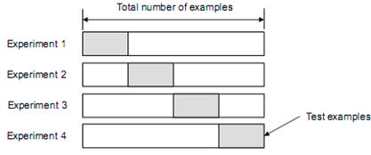
Cross Validation
- split data into three sub-sets
- train: to train the model
- validation: to tune hyper-parameters
- test: to evaluate prediction performance
Cross Validation
*** When do you not need a validation set? ***
*** Why do we need a train and a validation set? ***
*** Why do we need an extra test set? ***
*** Why could Rafael be upset with my plot? ***
fig_cross_val
Better Cross Validation
- Measurements without error bars do not exist!
- Split the data multiple times
k_values = range(1,150,10)

np.random.seed(seed=99)
random_seeds = np.random.randint(1000, size=50)

values = np.zeros((len(k_values),random_seeds.shape[0]))
for k, c_k in zip(k_values, range(len(k_values))):
    counter_rs = 0
    for rs,c_rs in zip(random_seeds, range(random_seeds.shape[0])):
        value = accuracy_for_k_val(k=k,x=x_sub_2d,y=y_sub,
                                   random_state=rs)
        values[c_k,c_rs] = value

sns.tsplot(values.T)
plt.xlabel('k')
plt.ylabel('accuracy')
plt.show()
k_values = range(1,150,10)

np.random.seed(seed=99)
random_seeds = np.random.randint(1000, size=50)

values = np.zeros((len(k_values),random_seeds.shape[0]))
for k, c_k in zip(k_values, range(len(k_values))):
    counter_rs = 0
    for rs,c_rs in zip(random_seeds, range(random_seeds.shape[0])):
        value = accuracy_for_k_val(k=k,x=x_sub_2d,y=y_sub,
                                   random_state=rs)
        values[c_k,c_rs] = value

sns.boxplot(values.T)
plt.xlabel('k')
plt.ylabel('accuracy')
plt.show()
Classifiers and Invariance
- digit recognition is
- translation invariant
- rotation invariant (a little bit)
Ways to Handle Invariance:
- add transformation to training data
- introduce canonical representation
- build into classifier
Rotation Invariance:

Tangent Space

Elements of Statistical Learning

Pattern Recognition Class
by Fred Hamprecht
on Youtube
http://www.youtube.com/playlist?list=PLuRaSnb3n4kRDZVU6wxPzGdx1CN12fn0w