Machine Learning with Python
We now have our data. We have sanitized it into a csv format. We have explored it.
Now lets try to predict some properties.
import pandas as pd

import matplotlib.pyplot as plt
## Load the data
# df = pd.read_csv('../data/mpdata.csv')
df = pd.read_csv('https://gitlab.com/costrouc/mse-machinelearning-notebooks/raw/master/data/mpdata.csv')
df.sample(5)
| material_id | energy | volume | nsites | energy_per_atom | pretty_formula | spacegroup | band_gap | density | total_magnetization | poisson_ratio | bulk_modulus_voigt | bulk_modulus_reuss | bulk_modulus_vrh | shear_modulus_voigt | shear_modulus_vrh | |
|---|---|---|---|---|---|---|---|---|---|---|---|---|---|---|---|---|
| 2621 | mp-559777 | -372.248991 | 732.106016 | 56 | -6.647303 | Na5Ca2Al(PO4)4 | 9 | 4.6496 | 2.730746 | -8.000000e-07 | NaN | NaN | NaN | NaN | NaN | NaN |
| 4063 | mp-603327 | -355.351207 | 654.019374 | 64 | -5.552363 | H3SNO3 | 61 | 5.1885 | 1.972148 | 1.312010e-02 | NaN | NaN | NaN | NaN | NaN | NaN |
| 5443 | mp-559382 | -17.053707 | 33.482124 | 3 | -5.684569 | CoO2 | 164 | 0.0000 | 4.509754 | 9.997688e-01 | NaN | NaN | NaN | NaN | NaN | NaN |
| 4616 | mp-558564 | -281.494573 | 681.185211 | 36 | -7.819294 | SiO2 | 12 | 5.5113 | 1.757625 | -1.510000e-05 | NaN | NaN | NaN | NaN | NaN | NaN |
| 2883 | mp-667374 | -1188.876440 | 2214.927434 | 168 | -7.076645 | NaAlSiO4 | 169 | 4.5414 | 2.555969 | 1.502800e-03 | NaN | NaN | NaN | NaN | NaN | NaN |
df.corr()
| energy | volume | nsites | energy_per_atom | spacegroup | band_gap | density | total_magnetization | poisson_ratio | bulk_modulus_voigt | bulk_modulus_reuss | bulk_modulus_vrh | shear_modulus_voigt | shear_modulus_vrh | |
|---|---|---|---|---|---|---|---|---|---|---|---|---|---|---|
| energy | 1.000000 | -0.852020 | -0.965198 | 0.345171 | 0.176241 | -0.378738 | 0.185483 | -0.121921 | 0.045966 | -0.080688 | -0.059895 | -0.071393 | -0.128289 | -0.056726 |
| volume | -0.852020 | 1.000000 | 0.862495 | -0.110264 | -0.162344 | 0.302136 | -0.309343 | 0.034127 | 0.000059 | -0.208067 | -0.187330 | -0.201073 | -0.110852 | -0.052474 |
| nsites | -0.965198 | 0.862495 | 1.000000 | -0.194668 | -0.217266 | 0.371992 | -0.248281 | 0.095329 | -0.032862 | -0.032160 | -0.028786 | -0.030992 | 0.042327 | 0.017493 |
| energy_per_atom | 0.345171 | -0.110264 | -0.194668 | 1.000000 | -0.038482 | -0.221015 | -0.334075 | -0.171508 | 0.051704 | -0.565429 | -0.465262 | -0.523804 | -0.434698 | -0.211633 |
| spacegroup | 0.176241 | -0.162344 | -0.217266 | -0.038482 | 1.000000 | -0.093678 | 0.250417 | -0.065560 | 0.028444 | 0.195654 | 0.205996 | 0.204483 | 0.113808 | 0.058407 |
| band_gap | -0.378738 | 0.302136 | 0.371992 | -0.221015 | -0.093678 | 1.000000 | -0.421409 | -0.220998 | -0.068310 | -0.266141 | -0.249368 | -0.262229 | -0.036694 | 0.000743 |
| density | 0.185483 | -0.309343 | -0.248281 | -0.334075 | 0.250417 | -0.421409 | 1.000000 | 0.322121 | 0.065513 | 0.501874 | 0.538017 | 0.529485 | 0.165460 | 0.086553 |
| total_magnetization | -0.121921 | 0.034127 | 0.095329 | -0.171508 | -0.065560 | -0.220998 | 0.322121 | 1.000000 | 0.023007 | 0.080165 | 0.089585 | 0.086458 | -0.006023 | -0.031027 |
| poisson_ratio | 0.045966 | 0.000059 | -0.032862 | 0.051704 | 0.028444 | -0.068310 | 0.065513 | 0.023007 | 1.000000 | -0.019499 | -0.022243 | -0.021264 | -0.143481 | 0.082642 |
| bulk_modulus_voigt | -0.080688 | -0.208067 | -0.032160 | -0.565429 | 0.195654 | -0.266141 | 0.501874 | 0.080165 | -0.019499 | 1.000000 | 0.930499 | 0.981958 | 0.676028 | 0.325090 |
| bulk_modulus_reuss | -0.059895 | -0.187330 | -0.028786 | -0.465262 | 0.205996 | -0.249368 | 0.538017 | 0.089585 | -0.022243 | 0.930499 | 1.000000 | 0.982977 | 0.598273 | 0.312095 |
| bulk_modulus_vrh | -0.071393 | -0.201073 | -0.030992 | -0.523804 | 0.204483 | -0.262229 | 0.529485 | 0.086458 | -0.021264 | 0.981958 | 0.982977 | 1.000000 | 0.647945 | 0.324180 |
| shear_modulus_voigt | -0.128289 | -0.110852 | 0.042327 | -0.434698 | 0.113808 | -0.036694 | 0.165460 | -0.006023 | -0.143481 | 0.676028 | 0.598273 | 0.647945 | 1.000000 | 0.460951 |
| shear_modulus_vrh | -0.056726 | -0.052474 | 0.017493 | -0.211633 | 0.058407 | 0.000743 | 0.086553 | -0.031027 | 0.082642 | 0.325090 | 0.312095 | 0.324180 | 0.460951 | 1.000000 |
plt.matshow(df.corr())
plt.colorbar()
<matplotlib.colorbar.Colorbar at 0x7fe83119e6d8>

Lets choose a very simple example to show methodology
How about we try to predict the energy_per_atom. You can see from the correlation plot that there are two very highly correlated values in purple.
We will simplify our model and only use the first four columns. Obviously volume is not usefull in the calculation but we want to see if our algorithm can automatically determine this.
simplified_df = df[['energy', 'volume', 'nsites', 'energy_per_atom']]
simplified_df.head(5)
| energy | volume | nsites | energy_per_atom | |
|---|---|---|---|---|
| 0 | -4.064600 | 11.852765 | 1 | -4.064600 |
| 1 | -16.382096 | 47.264158 | 4 | -4.095524 |
| 2 | -8.186959 | 23.617388 | 2 | -4.093479 |
| 3 | -4.064142 | 11.874703 | 1 | -4.064142 |
| 4 | -2.157191 | 603.475210 | 1 | -2.157191 |
All (99%) of machine learning algoritms need the data as arrays of floating point numbers. Scikit learn is no different. This is how easy it is to convery a pandas dataframe from a numpy array.
Not covered here but you most likely will need it at one point preprocessing data and how to handle categorical data.
# convert from pandas dataframe to numpy array
X = simplified_df[['energy', 'volume', 'nsites']].values
y = simplified_df['energy_per_atom'].values

print(X.shape, y.shape)
print(X[:3], y[:3])
(6928, 3) (6928,)
[[ -4.0645998   11.85276501   1.        ]
 [-16.38209642  47.26415795   4.        ]
 [ -8.18695876  23.61738783   2.        ]] [-4.0645998  -4.0955241  -4.09347938]
Scikit Learn
Very quick overview. Scikit learn provides a unified framework for working with machine learning algorithms. It includes classification, regression, clustering, dimensionality reduction, model tuning, pre and post processing of data.
Is that a lot? YES scikit learn is huge and you cannot expect to use and learn everything.
The flow chart gives some good advice for which algorithms to use for your problem. See their flow chart
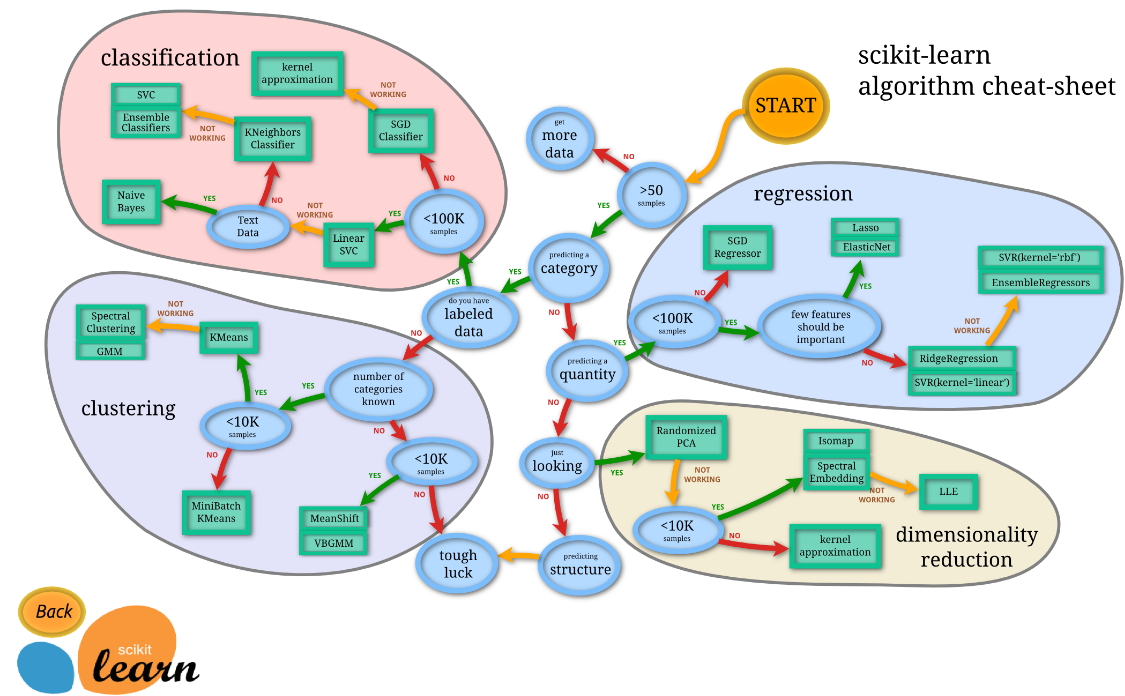
There are a ton of algoritms over 100! This is where sklearn really shines. All algorithms have the exact same api (this is the pseudocode).
from sklearn import MyImportantModel

model = MyImportantModel()
model.fit(X, y)
Once you have fit your model you can using is to predict future data.
y_predict = model.predict(X_predict)
We will be using a linear model to fit our data. Always start with the simplest model! That way you know what sort of improvement a complex one can get you.
# Lets use a simple linear model
from sklearn.linear_model import LinearRegression

model = LinearRegression()
from sklearn.model_selection import cross_val_predict

predicted =  cross_val_predict(model, X, y, cv=10)

fig, ax = plt.subplots()
ax.scatter(y, predicted, edgecolors=(0, 0, 0))
ax.plot([y.min(), y.max()], [y.min(), y.max()], 'k--', lw=4)
ax.set_xlabel('Measured')
ax.set_ylabel('Predicted')
plt.show()

# lest do the cross validation by hand
import sklearn
X_train, X_test, y_train, y_test = sklearn.model_selection.train_test_split(X, y, test_size=0.1)
model = LinearRegression()
model.fit(X_train, y_train)
LinearRegression(copy_X=True, fit_intercept=True, n_jobs=1, normalize=False)
y_predict = model.predict(X_test)

# calculate mean square error
sklearn.metrics.mean_squared_error(y_test, y_predict)
1.5827284267819932