Natural language inference: Models
__author__ = "Christopher Potts"
__version__ = "CS224u, Stanford, Spring 2019"
Contents
- Contents
- Overview
- Set-up
- Sparse feature representations
- Feature representations
- Model wrapper
- Assessment
- Sentence-encoding models
- Dense representations with a linear classifier
- Dense representations with a shallow neural network
- Sentence-encoding RNNs
- Other sentence-encoding model ideas
- Chained models
- Simple RNN
- Separate premise and hypothesis RNNs
- Attention mechanisms
- Error analysis with the MultiNLI annotations
- Other findings
- Exploratory exercises
Overview
This notebook defines and explores a number of models for NLI. The general plot is familiar from our work with the Stanford Sentiment Treebank:
- Models based on sparse feature representations
- Linear classifiers and feed-forward neural classifiers using dense feature representations
- Recurrent and tree-structured neural networks
The twist here is that, while NLI is another classification problem, the inputs have important high-level structure: a premise and a hypothesis. This invites exploration of a host of neural model designs:
In sentence-encoding models, the premise and hypothesis are analyzed separately, combined only for the final classification step.
In chained models, the premise is processed first, then the hypotheses, giving a unified representation of the pair.
NLI resembles sequence-to-sequence problems like machine translation and language modeling. The central modeling difference is that NLI doesn't produce an output sequence, but rather consumes two sequences to produce a label. Still, there are enough affinities that many ideas have been shared among these fields.
Set-up
See the previous notebook for set-up instructions for this unit.
from collections import Counter
from itertools import product
import numpy as np
import pandas as pd
from sklearn.linear_model import LogisticRegression
import torch
import torch.nn as nn
import torch.utils.data
from torch_model_base import TorchModelBase
from torch_rnn_classifier import TorchRNNClassifier, TorchRNNClassifierModel
from torch_shallow_neural_classifier import TorchShallowNeuralClassifier
from torch_rnn_classifier import TorchRNNClassifier
import nli
import os
import utils
GLOVE_HOME = os.path.join('data', 'glove.6B')

DATA_HOME = os.path.join("data", "nlidata")

SNLI_HOME = os.path.join(DATA_HOME, "snli_1.0")

MULTINLI_HOME = os.path.join(DATA_HOME, "multinli_1.0")

ANNOTATIONS_HOME = os.path.join(DATA_HOME, "multinli_1.0_annotations")
Sparse feature representations
We begin by looking at models based in sparse, hand-built feature representations. As in earlier units of the course, we will see that these models are competitive: easy to design, fast to optimize, and highly effective.
Feature representations
The guiding idea for NLI sparse features is that one wants to knit together the premise and hypothesis, so that the model can learn about their relationships rather than just about each part separately.
With word_overlap_phi, we just get the set of words that occur in both the premise and hypothesis.
def word_overlap_phi(t1, t2):
    """Basis for features for the words in both the premise and hypothesis.
    This tends to produce very sparse representations.

    Parameters
    ----------
    t1, t2 : `nltk.tree.Tree`
        As given by `str2tree`.

    Returns
    -------
    defaultdict
       Maps each word in both `t1` and `t2` to 1.

    """
    overlap = set([w1 for w1 in t1.leaves() if w1 in t2.leaves()])
    return Counter(overlap)
With word_cross_product_phi, we count all the pairs $(w_{1}, w_{1})$ where $w_{1}$ is a word from the premise and $w_{2}$ is a word from the hypothesis. This creates a very large feature space. These models are very strong right out of the box, and they can be supplemented with more fine-grained features.
def word_cross_product_phi(t1, t2):
    """Basis for cross-product features. This tends to produce pretty
    dense representations.

    Parameters
    ----------
    t1, t2 : `nltk.tree.Tree`
        As given by `str2tree`.

    Returns
    -------
    defaultdict
        Maps each (w1, w2) in the cross-product of `t1.leaves()` and
        `t2.leaves()` to its count. This is a multi-set cross-product
        (repetitions matter).

    """
    return Counter([(w1, w2) for w1, w2 in product(t1.leaves(), t2.leaves())])
Model wrapper
Our experiment framework is basically the same as the one we used for the Stanford Sentiment Treebank. Here, I actually use sst.fit_classifier_with_crossvalidation (from that unit) to create a wrapper around LogisticRegression for cross-validation of hyperparameters. At this point, I am not sure what parameters will be good for our NLI datasets, so this hyperparameter search is vital.
def fit_softmax_with_crossvalidation(X, y):
    """A MaxEnt model of dataset with hyperparameter cross-validation.

    Parameters
    ----------
    X : 2d np.array
        The matrix of features, one example per row.

    y : list
        The list of labels for rows in `X`.

    Returns
    -------
    sklearn.linear_model.LogisticRegression
        A trained model instance, the best model found.

    """
    basemod = LogisticRegression(
        fit_intercept=True,
        solver='liblinear',
        multi_class='auto')
    cv = 3
    param_grid = {'C': [0.4, 0.6, 0.8, 1.0],
                  'penalty': ['l1','l2']}
    best_mod = utils.fit_classifier_with_crossvalidation(
        X, y, basemod, cv, param_grid)
    return best_mod
Assessment
Because SNLI and MultiNLI are huge, we can't afford to do experiments on the full datasets all the time. Thus, we will mainly work within the training sets, using the train readers to sample smaller datasets that can then be divided for training and assessment.
Here, we sample 10% of the training examples. I set the random seed (random_state=42) so that we get consistency across the samples; setting random_state=None will give new random samples each time.
train_reader = nli.SNLITrainReader(
    SNLI_HOME, samp_percentage=0.10, random_state=42)
An experimental dataset can be built directly from the reader and a feature function:
dataset = nli.build_dataset(train_reader, word_overlap_phi)
dataset.keys()
dict_keys(['X', 'y', 'vectorizer', 'raw_examples'])
However, it's more efficient to use nli.experiment to bring all these pieces together. This wrapper will work for all the models we consider.
_ = nli.experiment(
    train_reader=nli.SNLITrainReader(SNLI_HOME, samp_percentage=0.10),
    phi=word_overlap_phi,
    train_func=fit_softmax_with_crossvalidation,
    assess_reader=None,
    random_state=42)
Best params: {'C': 0.8, 'penalty': 'l2'}
Best score: 0.415
Accuracy: 0.437
               precision    recall  f1-score   support

contradiction      0.445     0.673     0.536      5509
   entailment      0.462     0.382     0.418      5545
      neutral      0.387     0.256     0.309      5482

    micro avg      0.437     0.437     0.437     16536
    macro avg      0.432     0.437     0.421     16536
 weighted avg      0.432     0.437     0.421     16536
_ = nli.experiment(
    train_reader=nli.SNLITrainReader(SNLI_HOME, samp_percentage=0.10),
    phi=word_cross_product_phi,
    train_func=fit_softmax_with_crossvalidation,
    assess_reader=None,
    random_state=42)
Best params: {'C': 0.4, 'penalty': 'l1'}
Best score: 0.614
Accuracy: 0.626
               precision    recall  f1-score   support

contradiction      0.669     0.640     0.654      5473
   entailment      0.611     0.685     0.646      5356
      neutral      0.601     0.557     0.578      5558

    micro avg      0.626     0.626     0.626     16387
    macro avg      0.627     0.627     0.626     16387
 weighted avg      0.627     0.626     0.626     16387
As expected word_cross_product_phi is very strong. Let's take the hyperparameters chosen there and use them for an experiment in which we train on the entire training set and evaluate on the dev set; this seems like a good way to balance responsible search over hyperparameters with our resource limitations.
def fit_softmax_classifier_with_preselected_params(X, y):
    mod = LogisticRegression(
        fit_intercept=True,
        penalty='l1',
        solver='saga',  ## Required for penalty='ll'.
        multi_class='ovr',
        C=0.4)
    mod.fit(X, y)
    return mod
%%time
_ = nli.experiment(
    train_reader=nli.SNLITrainReader(SNLI_HOME, samp_percentage=1.0),
    assess_reader=nli.SNLIDevReader(SNLI_HOME, samp_percentage=1.0),
    phi=word_cross_product_phi,
    train_func=fit_softmax_classifier_with_preselected_params,
    random_state=None)
               precision    recall  f1-score   support

contradiction      0.762     0.729     0.745      3278
   entailment      0.708     0.795     0.749      3329
      neutral      0.716     0.657     0.685      3235

  avg / total      0.729     0.728     0.727      9842

CPU times: user 19min 17s, sys: 9.56 s, total: 19min 26s
Wall time: 19min 26s
This baseline is very similar to the one established in the original SNLI paper by Bowman et al. for models like this one.
Sentence-encoding models
We turn now to sentence-encoding models. The hallmark of these is that the premise and hypothesis get their own representation in some sense, and then those representations are combined to predict the label. Bowman et al. 2015 explore models of this form as part of introducing SNLI.
The feed-forward networks we used in the word-level bake-off are members of this family of models: each word was represented separately, and the concatenation of those representations was used as the input to the model.
Dense representations with a linear classifier
Perhaps the simplest sentence-encoding model sums (or averages, etc.) the word representations for the premise, does the same for the hypothesis, and concatenates those two representations for use as the input to a linear classifier.
Here's a diagram that is meant to suggest the full space of models of this form:

Here's an implementation of this model where
- The embedding is GloVe.
- The word representations are summed.
- The premise and hypothesis vectors are concatenated.
- A softmax classifier is used at the top.
glove_lookup = utils.glove2dict(
    os.path.join(GLOVE_HOME, 'glove.6B.50d.txt'))
def glove_leaves_phi(t1, t2, np_func=np.sum):
    """Represent `tree` as a combination of the vector of its words.

    Parameters
    ----------
    t1 : nltk.Tree
    t2 : nltk.Tree
    np_func : function (default: np.sum)
        A numpy matrix operation that can be applied columnwise,
        like `np.mean`, `np.sum`, or `np.prod`. The requirement is that
        the function take `axis=0` as one of its arguments (to ensure
        columnwise combination) and that it return a vector of a
        fixed length, no matter what the size of the tree is.

    Returns
    -------
    np.array

    """
    prem_vecs = _get_tree_vecs(t1, glove_lookup, np_func)
    hyp_vecs = _get_tree_vecs(t2, glove_lookup, np_func)
    return np.concatenate((prem_vecs, hyp_vecs))


def _get_tree_vecs(tree, lookup, np_func):
    allvecs = np.array([lookup[w] for w in tree.leaves() if w in lookup])
    if len(allvecs) == 0:
        dim = len(next(iter(lookup.values())))
        feats = np.zeros(dim)
    else:
        feats = np_func(allvecs, axis=0)
    return feats
_ = nli.experiment(
    train_reader=nli.SNLITrainReader(SNLI_HOME, samp_percentage=0.10),
    phi=glove_leaves_phi,
    train_func=fit_softmax_with_crossvalidation,
    assess_reader=None,
    random_state=42,
    vectorize=False)  # Ask `experiment` not to featurize; we did it already.
Best params: {'C': 0.4, 'penalty': 'l1'}
Best score: 0.504
Accuracy: 0.502
               precision    recall  f1-score   support

contradiction      0.495     0.464     0.479      5499
   entailment      0.484     0.563     0.521      5536
      neutral      0.533     0.478     0.504      5525

    micro avg      0.502     0.502     0.502     16560
    macro avg      0.504     0.502     0.501     16560
 weighted avg      0.504     0.502     0.501     16560
Dense representations with a shallow neural network
A small tweak to the above is to use a neural network instead of a softmax classifier at the top:
def fit_shallow_neural_classifier_with_crossvalidation(X, y):
    basemod = TorchShallowNeuralClassifier(max_iter=1000)
    cv = 3
    param_grid = {'hidden_dim': [25, 50, 100]}
    best_mod = utils.fit_classifier_with_crossvalidation(
        X, y, basemod, cv, param_grid)
    return best_mod
_ = nli.experiment(
    train_reader=nli.SNLITrainReader(SNLI_HOME, samp_percentage=0.10),
    phi=glove_leaves_phi,
    train_func=fit_shallow_neural_classifier_with_crossvalidation,
    assess_reader=None,
    random_state=42,
    vectorize=False)  # Ask `experiment` not to featurize; we did it already.
Finished epoch 1000 of 1000; error is 32.213042318820959
Best params: {'hidden_dim': 25}
Best score: 0.514
Accuracy: 0.535
               precision    recall  f1-score   support

contradiction      0.541     0.476     0.506      5364
   entailment      0.522     0.646     0.577      5608
      neutral      0.547     0.478     0.510      5471

    micro avg      0.535     0.535     0.535     16443
    macro avg      0.537     0.533     0.531     16443
 weighted avg      0.537     0.535     0.532     16443
Sentence-encoding RNNs
A more sophisticated sentence-encoding model processes the premise and hypothesis with separate RNNs and uses the concatenation of their final states as the basis for the classification decision at the top:
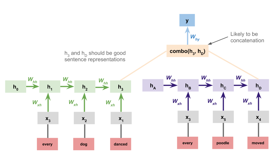
It is relatively straightforward to extend torch_rnn_classifier so that it can handle this architecture:
A sentence-encoding dataset
Whereas torch_rnn_classifier.TorchRNNDataset creates batches that consist of (sequence, sequence_length, label) triples, the sentence encoding model requires us to double the first two components. The most important features of this is collate_fn, which determines what the batches look like:
class TorchRNNSentenceEncoderDataset(torch.utils.data.Dataset):
    def __init__(self, sequences, seq_lengths, y):
        self.prem_seqs, self.hyp_seqs = sequences
        self.prem_lengths, self.hyp_lengths = seq_lengths
        self.y = y
        assert len(self.prem_seqs) == len(self.y)

    @staticmethod
    def collate_fn(batch):
        X_prem, X_hyp, prem_lengths, hyp_lengths, y = zip(*batch)
        prem_lengths = torch.LongTensor(prem_lengths)
        hyp_lengths = torch.LongTensor(hyp_lengths)
        y = torch.LongTensor(y)
        return (X_prem, X_hyp), (prem_lengths, hyp_lengths), y

    def __len__(self):
        return len(self.prem_seqs)

    def __getitem__(self, idx):
        return (self.prem_seqs[idx], self.hyp_seqs[idx],
                self.prem_lengths[idx], self.hyp_lengths[idx],
                self.y[idx])
A sentence-encoding model
With TorchRNNSentenceEncoderClassifierModel, we subclass torch_rnn_classifier.TorchRNNClassifierModel and make use of many of its parameters. The changes:
- We add an attribute
self.hypothesis_rnnfor encoding the hypothesis. (The super class hasself.rnn, which we use for the premise.) - The
forwardmethod concatenates the final states from the premise and hypothesis, and they are the input to the classifier layer, which is unchanged from before but how accepts inputs that are double the size.
class TorchRNNSentenceEncoderClassifierModel(TorchRNNClassifierModel):
    def __init__(self, vocab_size, embed_dim, embedding, use_embedding,
            hidden_dim, output_dim, bidirectional, device):
        super(TorchRNNSentenceEncoderClassifierModel, self).__init__(
            vocab_size, embed_dim, embedding, use_embedding,
            hidden_dim, output_dim, bidirectional, device)
        self.hypothesis_rnn = nn.LSTM(
            input_size=self.embed_dim,
            hidden_size=hidden_dim,
            batch_first=True,
            bidirectional=self.bidirectional)
        if bidirectional:
            classifier_dim = hidden_dim * 2 * 2
        else:
            classifier_dim = hidden_dim * 2
        self.classifier_layer = nn.Linear(
            classifier_dim, output_dim)

    def forward(self, X, seq_lengths):
        X_prem, X_hyp = X
        prem_lengths, hyp_lengths = seq_lengths
        prem_state = self.rnn_forward(X_prem, prem_lengths, self.rnn)
        hyp_state = self.rnn_forward(X_hyp, hyp_lengths, self.hypothesis_rnn)
        state = torch.cat((prem_state, hyp_state), dim=1)
        logits = self.classifier_layer(state)
        return logits
A sentence-encoding model interface
Finally, we subclass TorchRNNClassifier. Here, just need to redefine three methods: build_dataset and build_graph to make use of the new components above, and predict_proba so that it deals with the premise/hypothesis shape of new inputs.
class TorchRNNSentenceEncoderClassifier(TorchRNNClassifier):

    def build_dataset(self, X, y):
        X_prem, X_hyp = zip(*X)
        X_prem, prem_lengths = self._prepare_dataset(X_prem)
        X_hyp, hyp_lengths = self._prepare_dataset(X_hyp)
        return TorchRNNSentenceEncoderDataset(
            (X_prem, X_hyp), (prem_lengths, hyp_lengths), y)

    def build_graph(self):
        return TorchRNNSentenceEncoderClassifierModel(
            len(self.vocab),
            embedding=self.embedding,
            embed_dim=self.embed_dim,
            use_embedding=self.use_embedding,
            hidden_dim=self.hidden_dim,
            output_dim=self.n_classes_,
            bidirectional=self.bidirectional,
            device=self.device)

    def predict_proba(self, X):
        with torch.no_grad():
            X_prem, X_hyp = zip(*X)
            X_prem, prem_lengths = self._prepare_dataset(X_prem)
            X_hyp, hyp_lengths = self._prepare_dataset(X_hyp)
            preds = self.model((X_prem, X_hyp), (prem_lengths, hyp_lengths))
            preds = torch.softmax(preds, dim=1).cpu().numpy()
            return preds
Simple example
This toy problem illustrates how this works in detail:
def simple_example():
    vocab = ['a', 'b', '$UNK']

    # Reversals are good, and other pairs are bad:
    train = [
        [(list('ab'), list('ba')), 'good'],
        [(list('aab'), list('baa')), 'good'],
        [(list('abb'), list('bba')), 'good'],
        [(list('aabb'), list('bbaa')), 'good'],
        [(list('ba'), list('ba')), 'bad'],
        [(list('baa'), list('baa')), 'bad'],
        [(list('bba'), list('bab')), 'bad'],
        [(list('bbaa'), list('bbab')), 'bad'],
        [(list('aba'), list('bab')), 'bad']]

    test = [
        [(list('baaa'), list('aabb')), 'bad'],
        [(list('abaa'), list('baaa')), 'bad'],
        [(list('bbaa'), list('bbaa')), 'bad'],
        [(list('aaab'), list('baaa')), 'good'],
        [(list('aaabb'), list('bbaaa')), 'good']]

    mod = TorchRNNSentenceEncoderClassifier(
        vocab,
        max_iter=100,
        embed_dim=50,
        hidden_dim=50)

    X, y = zip(*train)
    mod.fit(X, y)

    X_test, y_test = zip(*test)
    preds = mod.predict(X_test)

    print("\nPredictions:")
    for ex, pred, gold in zip(X_test, preds, y_test):
        score = "correct" if pred == gold else "incorrect"
        print("{0:>6} {1:>6} - predicted: {2:>4}; actual: {3:>4} - {4}".format(
            "".join(ex[0]), "".join(ex[1]), pred, gold, score))
simple_example()
Finished epoch 100 of 100; error is 2.7179718017578125e-05
Predictions:
  baaa   aabb - predicted:  bad; actual:  bad - correct
  abaa   baaa - predicted:  bad; actual:  bad - correct
  bbaa   bbaa - predicted:  bad; actual:  bad - correct
  aaab   baaa - predicted: good; actual: good - correct
 aaabb  bbaaa - predicted: good; actual: good - correct
Example SNLI run
def sentence_encoding_rnn_phi(t1, t2):
    """Map `t1` and `t2` to a pair of lits of leaf nodes."""
    return (t1.leaves(), t2.leaves())
def get_sentence_encoding_vocab(X, n_words=None):
    wc = Counter([w for pair in X for ex in pair for w in ex])
    wc = wc.most_common(n_words) if n_words else wc.items()
    vocab = {w for w, c in wc}
    vocab.add("$UNK")
    return sorted(vocab)
def fit_sentence_encoding_rnn(X, y):
    vocab = get_sentence_encoding_vocab(X, n_words=10000)
    mod = TorchRNNSentenceEncoderClassifier(
        vocab, hidden_dim=50, max_iter=50)
    mod.fit(X, y)
    return mod
_ = nli.experiment(
    train_reader=nli.SNLITrainReader(SNLI_HOME, samp_percentage=0.10),
    phi=sentence_encoding_rnn_phi,
    train_func=fit_sentence_encoding_rnn,
    assess_reader=None,
    random_state=42,
    vectorize=False)
Finished epoch 50 of 50; error is 0.009828846727032214
               precision    recall  f1-score   support

contradiction      0.542     0.540     0.541      5458
   entailment      0.567     0.569     0.568      5425
      neutral      0.544     0.545     0.545      5528

    micro avg      0.551     0.551     0.551     16411
    macro avg      0.551     0.551     0.551     16411
 weighted avg      0.551     0.551     0.551     16411
Other sentence-encoding model ideas
Given that we already explored tree-structured neural networks (TreeNNs), it's natural to consider these as the basis for sentence-encoding NLI models:
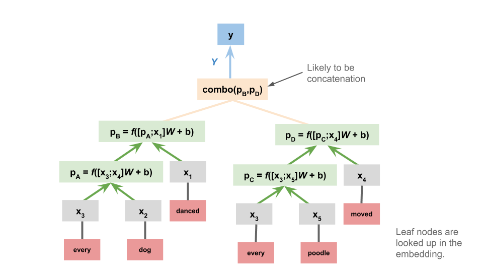
And this is just the begnning: any model used to represent sentences is presumably a candidate for use in sentence-encoding NLI!
Chained models
The final major class of NLI designs we look at are those in which the premise and hypothesis are processed sequentially, as a pair. These don't deliver representations of the premise or hypothesis separately. They bear the strongest resemblance to classic sequence-to-sequence models.
Simple RNN
In the simplest version of this model, we just concatenate the premise and hypothesis. The model itself is identical to the one we used for the Stanford Sentiment Treebank:
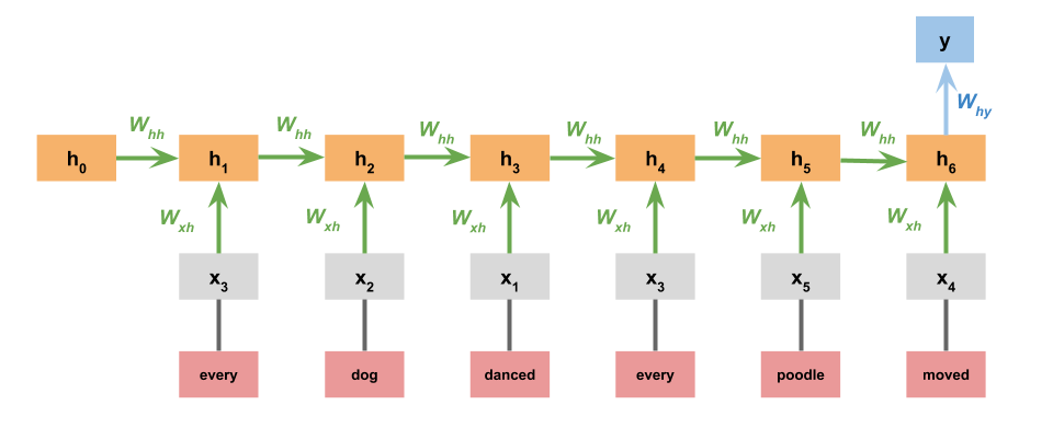
To implement this, we can use TorchRNNClassifier out of the box. We just need to concatenate the leaves of the premise and hypothesis trees:
def simple_chained_rep_rnn_phi(t1, t2):
    """Map `t1` and `t2` to a single list of leaf nodes.

    A slight variant might insert a designated boundary symbol between
    the premise leaves and the hypothesis leaves. Be sure to add it to
    the vocab in that case, else it will be $UNK.
    """
    return t1.leaves() + t2.leaves()
Here's a quick evaluation, just to get a feel for this model:
def fit_simple_chained_rnn(X, y):
    vocab = utils.get_vocab(X, n_words=10000)
    mod = TorchRNNClassifier(vocab, hidden_dim=50, max_iter=50)
    mod.fit(X, y)
    return mod
_ = nli.experiment(
    train_reader=nli.SNLITrainReader(SNLI_HOME, samp_percentage=0.10),
    phi=simple_chained_rep_rnn_phi,
    train_func=fit_simple_chained_rnn,
    assess_reader=None,
    random_state=42,
    vectorize=False)
Finished epoch 50 of 50; error is 1.9316425714641814
Accuracy: 0.561
               precision    recall  f1-score   support

contradiction      0.564     0.544     0.554      5517
   entailment      0.581     0.566     0.573      5441
      neutral      0.541     0.573     0.557      5534

    micro avg      0.561     0.561     0.561     16492
    macro avg      0.562     0.561     0.561     16492
 weighted avg      0.562     0.561     0.561     16492
Separate premise and hypothesis RNNs
A natural variation on the above is to give the premise and hypothesis each their own RNN:
This greatly increases the number of parameters, but it gives the model more chances to learn that appearing in the premise is different from appearing in the hypothesis. One could even push this idea further by giving the premise and hypothesis their own embeddings as well. One could implement this easily by modifying the sentence-encoder version defined above.
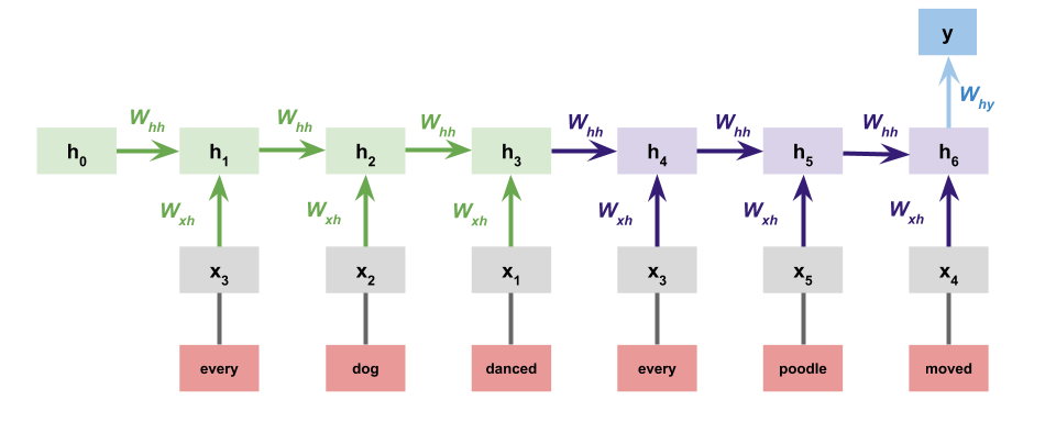
Attention mechanisms
Many of the best-performing systems in the SNLI leaderboard use attention mechanisms to help the model learn important associations between words in the premise and words in the hypothesis. I believe Rocktäschel et al. (2015) were the first to explore such models for NLI.
For instance, if puppy appears in the premise and dog in the conclusion, then that might be a high-precision indicator that the correct relationship is entailment.
This diagram is a high-level schematic for adding attention mechanisms to a chained RNN model for NLI:

Since TensorFlow will handle the details of backpropagation, implementing these models is largely reduced to figuring out how to wrangle the states of the model in the desired way.
Error analysis with the MultiNLI annotations
The annotations included with the MultiNLI corpus create some powerful yet easy opportunities for error analysis right out of the box. This section illustrates how to make use of them with models you've trained.
First, we train a sentence-encoding model on a sample of the MultiNLI data, just for illustrative purposes:
rnn_multinli_experiment = nli.experiment(
    train_reader=nli.MultiNLITrainReader(MULTINLI_HOME, samp_percentage=0.10),
    phi=sentence_encoding_rnn_phi,
    train_func=fit_sentence_encoding_rnn,
    assess_reader=None,
    random_state=42,
    vectorize=False)
Finished epoch 50 of 50; error is 0.024059262155788027
Accuracy: 0.426
               precision    recall  f1-score   support

contradiction      0.476     0.467     0.471      3888
   entailment      0.400     0.398     0.399      3991
      neutral      0.406     0.415     0.410      3929

    micro avg      0.426     0.426     0.426     11808
    macro avg      0.427     0.427     0.427     11808
 weighted avg      0.427     0.426     0.427     11808
The return value of nli.experiment contains the information we need to make predictions on new examples.
Next, we load in the 'matched' condition annotations ('mismatched' would work as well):
matched_ann_filename = os.path.join(
    ANNOTATIONS_HOME,
    "multinli_1.0_matched_annotations.txt")
matched_ann = nli.read_annotated_subset(
    matched_ann_filename, MULTINLI_HOME)
The following function uses rnn_multinli_experiment to make predictions on annotated examples, and harvests some other information that is useful for error analysis:
def predict_annotated_example(ann, experiment_results):
    model = experiment_results['model']
    phi = experiment_results['phi']
    ex = ann['example']
    prem = ex.sentence1_parse
    hyp = ex.sentence2_parse
    feats = phi(prem, hyp)
    pred = model.predict([feats])[0]
    gold = ex.gold_label
    data = {cat: True for cat in ann['annotations']}
    data.update({'gold': gold, 'prediction': pred, 'correct': gold == pred})
    return data
Finally, this function applies predict_annotated_example to a collection of annotated examples and puts the results in a pd.DataFrame for flexible analysis:
def get_predictions_for_annotated_data(anns, experiment_results):
    data = []
    for ex_id, ann in anns.items():
        results = predict_annotated_example(ann, experiment_results)
        data.append(results)
    return pd.DataFrame(data)
ann_analysis_df = get_predictions_for_annotated_data(
    matched_ann, rnn_multinli_experiment)
With ann_analysis_df, we can see how the model does on individual annotation categories:
pd.crosstab(ann_analysis_df['correct'], ann_analysis_df['#MODAL'])
| #MODAL | True |
|---|---|
| correct | |
| False | 75 |
| True | 69 |
Other findings
A high-level lesson of the SNLI leaderboard is that one can do extremely well with simple neural models whose hyperparameters are selected via extensive cross-validation. This is mathematically interesting but might be dispiriting to those of us without vast resources to devote to these computations! (On the flip side, cleverly designed linear models or ensembles with sparse feature representations might beat all of these entrants with a fraction of the computational budget.)
In an outstanding project for this course in 2016, Leonid Keselman observed that one can do much better than chance on SNLI by processing only the hypothesis. This relates to observations we made in the word-level homework/bake-off about how certain terms will tend to appear more on the right in entailment pairs than on the left. Last year, a number of groups independently (re-)discovered this fact and published analyses: Poliak et al. 2018, Tsuchiya 2018, Gururangan et al. 2018.
As we pointed out at the start of this unit, Dagan et al. (2006) pitched NLI as a general-purpose NLU task. We might then hope that the representations we learn on this task will transfer to others. So far, the evidence for this is decidedly mixed. I suspect the core scientific idea is sound, but that we still lack the needed methods for doing transfer learning.
For SNLI, we seem to have entered the inevitable phase in machine learning problems where ensembles do best.
Exploratory exercises
These are largely meant to give you a feel for the material, but some of them could lead to projects and help you with future work for the course. These are not for credit.
When we feed dense representations to a simple classifier, what is the effect of changing the combination functions (e.g., changing
sumtomean; changingconcatenatetodifference)? What happens if we swap outLogisticRegressionfor, say, an sklearn.ensemble.RandomForestClassifier instance?Implement the Separate premise and hypothesis RNN and evaluate it, comparing in particular against the version that simply concatenates the premise and hypothesis. Does having all these additional parameters pay off? Do you need more training examples to start to see the value of this idea?
The illustrations above all use SNLI. It is worth experimenting with MultiNLI as well. It has both matched and mismatched dev sets. It's also interesting to think about combining SNLI and MultiNLI, to get additional training instances, to push the models to generalize more, and to assess transfer learning hypotheses.