Plotting and curve fitting
In this lesson, we will create some plots and also fit mathematic models to data using curve-fitting techniques. By the end of the lesson, you will be able to:
- create a plot with multiple curves, labelled axes, and a legend.
- fit a mathematical curve to experimental data using the linear least squares method.
Creating plots
To create plots, we are going to use a package called pyplot, which is part of a package called matplotlib. Full documentation can be found on matplotlib.org.
You can install the library in Thonny by clicking on Tools->Manage packages and typing matplotlib into the text box at the top.
Note: if running this notebook online, you need to install numpy by running the cell below:
!pip3 install matplotlib
To use pyplot in our scripts, we import it as follows:
import matplotlib.pyplot as plt
Consider the following data from a tensile test on specimen:
Force (N) Length (mm)
0 25.4
13031 25.474
21485 25.515
31963 25.575
34727 25.615
37119 25.693
37960 25.752
39550 25.978
40758 26.419
40986 26.502
41076 26.600
41255 26.728
41481 27.130
41564 27.441
We can plot the data above as follows using the plot() command.
import matplotlib.pyplot as plt
import numpy as np

force = np.array([0, 13031, 21485, 31963, 34727, 37119, 37960, 39550, 40758, 40986, 41076, 41255, 41481, 41564])
sample_length = np.array([25.4, 25.474, 25.515, 25.575, 25.615, 25.693, 25.752, 25.978, 26.419, 26.502, 26.6, 26.728, 27.13, 27.441])

plt.ion() # Allows you to use the shell with plot open; to turn it off use plt.ioff()
plt.plot(sample_length, force)
# plt.show()  # Needed when plt.off() is used
Typically, we plot experimental data as points and not lines.
plt.plot(sample_length, force, 'o') # This plots each point as a circle
plt.plot(sample_length, force, 'rs') # This plots each point as a red square
plt.xlabel('Length (mm)')
plt.ylabel('Force (N)')
You can add more plots to the figure by repeatedly using the plot command. Let's add a second set of data to the figure.
force_2 = np.array([0, 12900, 20410, 30364, 33337, 35263, 37200, 38759, 39127, 40576, 39843, 40429, 40236, 41148])
sample_length_2 = np.array([25.4, 25.474, 25.515, 25.575, 25.615, 25.95, 26.01, 25.978, 26.684, 26.502, 26.866, 26.728, 27.13, 27.716])

plt.plot(sample_length_2, force_2, 'bv') # Adds the second set as blue triangles
Finally, we can add a legend to the plot using legend.
plt.legend(('Data set 1','Data set 2'), loc='best') # The best option positions the legend box in the least obtrusive location
Exercise
The velocity of an object was measured every second for 10 seconds. A model of the motion was created that best fit the experimental data.
Time (s) 0 1 2 3 4 5 6 7 8 9 10
Experimental velocity (m/s) 0 0.23 0.54 0.81 1.04 1.25 1.395 1.61 2.18 2.4075 2.55
Model velocity (m/s) 0 0.25 0.5 0.75 1 1.25 1.5 1.75 2 2.25 2.5
Plot the experimental and model data on the one figure. Include axes labels and legend. Plot the experimental data as points and the model data as a solid line.
Curve fitting using linear least squares method
Frequently in engineering we conduct experiments where we observe various parameters over time (e.g. temperature, pressure, load). From the experimental data, we can create mathematical models that describe the observed phenomenon. Curve-fitting is one method of creating these models.
Curve fitting is a a procedure where the parameters of a mathematical equation of a model are adjusted so that the model is best-fit to the experimental data. The resulting model curve does not go through all (or sometimes any) of the experimental data points. An overall best fit is achieved.
There are many different methods of curve-fitting, which are suited to different situations. we are going to examine the method of least squares and us it to find linear equations that best fit experimental data. Consider the following plot of experimental data.
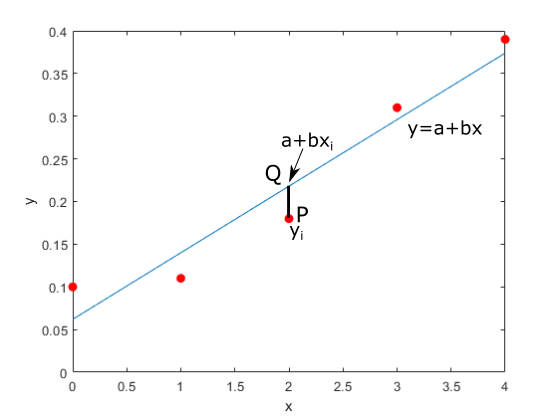
From observation, a linear equation can be used to best-fit the data. The equation takes the form: $$y=a+bx$$ Our goal is to determine the parameters $a$ and $b$.
Consider the points P and Q in the plot above. P is the experimental value at $x_i$ and Q is the corresponding model value at $x_i$. The residual or error is the distance $PQ$, which is given by
$$PQ=y_i-(a+bx_i)$$From this
$$PQ^2=(y_i-a-bx_i)^2)$$If we sum up all the residuals or errors for all the data points we get
$$S=\sum\limits_{i=1}^{n}(y_i-a-bx_i)^2)$$We want to find $a$ and $b$ such that $S$ is a minimum. $a$ and $b$ can be shown to be
$$a=\frac{\sum\limits_{i=1}^{n}y_i-b\sum\limits_{i=1}^{n}x_i}{n}$$$$b=\frac{\sum\limits_{i=1}^{n}x_iy_i-\frac{1}{n}\sum\limits_{i=1}^{n}x_i\sum\limits_{i=1}^{n}y_i}{\sum\limits_{i=1}^{n}x_i^2-\frac{1}{n}\left(\sum\limits_{i=1}^{n}x_i\right)^2}$$Exercise
Write a function that finds the parameters $a$ and $b$. The function definition is:
def linear_least_squares(xi, yi):

    n = len(Texp)

    b =

    a =

    return a, b
Consider the following data:
import numpy as np

xi = np.array([0, 1, 2, 3, 4])
yi = np.array([0.1, 0.11, 0.18, 0.31, 0.39])
Find the linear equation that best fits that data. Show the experimental data and the equation on the one plot.
Problem 1
According to Charles' Law for an ideal gas at constant volume, a linear relationship exists between the pressure P and temperature T. The following results are from heating a gas in a sealed container.
T ($^o$C) 0 10 20 30 40 50 60 70 80 90 100
P (atm) 0.94 0.96 1.00 1.05 1.07 1.09 1.14 1.17 1.21 1.24 1.28
- Determine the linear fit equation.
- Plot the experimental data with the model equation superimposed on it. Include axes labels, and legend.
- Extrapolate the linear fit equation until it crosses the horizontal line. What is the temperature when the pressure is zero?