Higgs decay to two photons
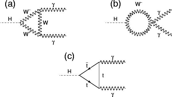
The Standard Model predicted the decay of the [Higgs bosons](https://en.wikipedia.org/wiki/Higgs_boson) into photons. The process is depicted by the diagrams below:
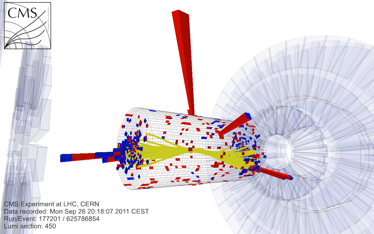
 At the [Large Hadron Collider](https://en.wikipedia.org/wiki/Large_Hadron_Collider), this process has been measured. This figure shows how an Higgs boson decay looks in the CMS detector:
 This ROOTbook illustrates a simplified fitting procedure aiming to identify the peak due to the Higgs boson decay over the exponentially falling background.
Importing input data into a ROOT file
First of all we import the input data, here simplistically stored into a text file, into a ROOT file.
TTree tree("HiggsTree","The tree cont");
auto nevt = tree.ReadFile("Hgg.txt","x");
if (nevt <= 0) {
    Error("fitHgg","Error reading data from input file ");
    }
std::cout << "Read " << nevt << " events from the file." << std::endl;
Read 30770 events from the file.
Modelling the distributions with RooFit
ROOT provides a tool for rich modelling of statistical distributions: RooFit. We now create a RooFit model using the RooWorkspace factory: a tool which allow to express complex entities with a convenient syntax.
RooWorkspace w("Workspace for the Higgs fit");
w.factory("x[110,160]");  // invariant mass

// Backround Model
w.factory("nbackground[10000, 0, 10000]");
w.var("nbackground")->setVal(nevt);
w.var("nbackground")->setMin(0.1*nevt);
w.var("nbackground")->setMax(10*nevt);

// Create exponential distribution characterised by two components
w.factory("a1[ 7.5, -500, 500]");
w.factory("a2[-1.5, -500, 500]");
w.factory("expr::z('-(a1*x/100 + a2*(x/100)^2)', a1, a2, x)");
w.factory("Exponential::bmodel(z, 1)");

// Signal Model
w.factory("nsignal[100, 0.0, 1000.0]");
w.factory("mass[130, 110, 150]");
w.factory("width[1, 0.5, 5]");
w.factory("Gaussian::smodel(x, mass, width)");

// Signal + Background Model
w.factory("SUM::model(nbackground*bmodel, nsignal*smodel)");
RooFit v3.60 -- Developed by Wouter Verkerke and David Kirkby
                Copyright (C) 2000-2013 NIKHEF, University of California & Stanford University
                All rights reserved, please read http://roofit.sourceforge.net/license.txt
Extract the signal and signal+background model from the workspace:
auto smodel = w.pdf("smodel");
auto model = w.pdf("model");
auto x = w.var("x");
We create now the RooFit data set importing the data from the ROOT tree
RooDataSet dataset("data","data",*x,RooFit::Import(tree) )
[#1] INFO:Eval -- RooAbsReal::attachToTree(x) TTree Float_t branch x will be converted to double precision
(RooDataSet &) Name: data Title: data
The workspace can be printed on screen: this is very useful to inspect the models created.
w.Print();
RooWorkspace(Workspace for the Higgs fit) Workspace for the Higgs fit contents

variables
---------
(a1,a2,mass,nbackground,nsignal,width,x)

p.d.f.s
-------
RooExponential::bmodel[ x=z c=1 ] = 0.000616625
RooAddPdf::model[ nbackground * bmodel + nsignal * smodel ] = 0.000610556
RooGaussian::smodel[ x=x mean=mass sigma=width ] = 3.72665e-06

functions
--------
RooFormulaVar::z[ actualVars=(a1,a2,x) formula="-(a1*x/100+a2*(x/100)^2)" ] = -7.39125
Fit of the Data
The fitting procedure results in quite some output. It is important to learn how to read the output of a fit, for example the value of the parameters, their uncertainties, the correlation matrix and the status of the fitting procedure.
** Be patient: the fit is unbinned and can take a while **
auto r = model->fitTo(dataset, RooFit::Minimizer("Minuit"),RooFit::Save(true), RooFit::Offset(true));
[#1] INFO:Minization -- p.d.f. provides expected number of events, including extended term in likelihood.
[#1] INFO:NumericIntegration -- RooRealIntegral::init(bmodel_Int[x]) using numeric integrator RooIntegrator1D to calculate Int(x)
[#1] INFO:Minization -- RooMinimizer::optimizeConst: activating const optimization
[#1] INFO:NumericIntegration -- RooRealIntegral::init(bmodel_Int[x]) using numeric integrator RooIntegrator1D to calculate Int(x)
[#1] INFO:Minization --  The following expressions will be evaluated in cache-and-track mode: (bmodel,smodel)
 **********
 **    1 **SET PRINT           1
 **********
 **********
 **    2 **SET NOGRAD
 **********
 PARAMETER DEFINITIONS:
    NO.   NAME         VALUE      STEP SIZE      LIMITS
     1 a1           7.50000e+00  1.00000e+02   -5.00000e+02  5.00000e+02
     2 a2          -1.50000e+00  1.00000e+02   -5.00000e+02  5.00000e+02
     3 mass         1.30000e+02  4.00000e+00    1.10000e+02  1.50000e+02
     4 nbackground   1.00000e+04  3.46150e+03    3.07700e+03  3.07700e+05
     5 nsignal      1.00000e+02  5.00000e+01    0.00000e+00  1.00000e+03
     6 width        1.00000e+00  2.50000e-01    5.00000e-01  5.00000e+00
 **********
 **    3 **SET ERR         0.5
 **********
 **********
 **    4 **SET PRINT           1
 **********
 **********
 **    5 **SET STR           1
 **********
 NOW USING STRATEGY  1: TRY TO BALANCE SPEED AGAINST RELIABILITY
 **********
 **    6 **MIGRAD        3000           1
 **********
 FIRST CALL TO USER FUNCTION AT NEW START POINT, WITH IFLAG=4.
[#1] INFO:Minization -- RooNLLVar::evaluatePartition(nll_model_data) first = 0 last = 30770 Likelihood offset now set to -156454
 START MIGRAD MINIMIZATION.  STRATEGY  1.  CONVERGENCE WHEN EDM .LT. 1.00e-03
 FCN=-382.008 FROM MIGRAD    STATUS=INITIATE      121 CALLS         122 TOTAL
                     EDM= unknown      STRATEGY= 1      NO ERROR MATRIX
  EXT PARAMETER               CURRENT GUESS       STEP         FIRST
  NO.   NAME      VALUE            ERROR          SIZE      DERIVATIVE
   1  a1           7.50000e+00   1.00000e+02   0.00000e+00   8.25702e+04
   2  a2          -1.50000e+00   1.00000e+02   0.00000e+00   2.24355e+05
   3  mass         1.24328e+02   4.00000e+00   0.00000e+00   4.66358e+01
   4  nbackground   1.00000e+04   3.46150e+03   0.00000e+00  -9.08535e+04
   5  nsignal      3.12951e+02   5.00000e+01   3.64250e-01  -6.58428e+02
   6  width        1.00000e+00   2.50000e-01   0.00000e+00  -1.31987e+02
                               ERR DEF= 0.5
 MIGRAD MINIMIZATION HAS CONVERGED.
 MIGRAD WILL VERIFY CONVERGENCE AND ERROR MATRIX.
 COVARIANCE MATRIX CALCULATED SUCCESSFULLY
 FCN=-13661.8 FROM MIGRAD    STATUS=CONVERGED     393 CALLS         394 TOTAL
                     EDM=2.73773e-06    STRATEGY= 1      ERROR MATRIX ACCURATE
  EXT PARAMETER                                   STEP         FIRST
  NO.   NAME      VALUE            ERROR          SIZE      DERIVATIVE
   1  a1           8.62159e+00   7.99131e-01   6.71813e-06   3.95343e+00
   2  a2          -2.02240e+00   3.02257e-01   2.53440e-06   1.05738e+01
   3  mass         1.24043e+02   5.15995e-01   2.10145e-03  -5.18608e-02
   4  nbackground   3.04968e+04   1.94972e+02   1.62355e-04   1.89450e-01
   5  nsignal      2.73230e+02   8.78269e+01   1.19000e-02   4.11368e-03
   6  width        1.48353e+00   4.52588e-01   1.61020e-02   1.06792e-03
                               ERR DEF= 0.5
 EXTERNAL ERROR MATRIX.    NDIM=  25    NPAR=  6    ERR DEF=0.5
  6.386e-01 -2.412e-01  4.880e-03 -2.017e+01 -2.020e+01  5.434e-02
 -2.412e-01  9.136e-02 -1.149e-03  7.853e+00  7.866e+00 -2.129e-02
  4.880e-03 -1.149e-03  2.663e-01  8.075e+00  8.083e+00 -5.954e-02
 -2.017e+01  7.853e+00  8.075e+00  3.801e+04  7.529e+03 -2.255e+01
 -2.020e+01  7.866e+00  8.083e+00  7.529e+03  7.816e+03 -2.257e+01
  5.434e-02 -2.129e-02 -5.954e-02 -2.255e+01 -2.257e+01  2.090e-01
 PARAMETER  CORRELATION COEFFICIENTS
       NO.  GLOBAL      1      2      3      4      5      6
        1  0.99864   1.000 -0.999  0.012 -0.129 -0.286  0.149
        2  0.99865  -0.999  1.000 -0.007  0.133  0.294 -0.154
        3  0.26833   0.012 -0.007  1.000  0.080  0.177 -0.252
        4  0.43699  -0.129  0.133  0.080  1.000  0.437 -0.253
        5  0.66859  -0.286  0.294  0.177  0.437  1.000 -0.558
        6  0.57982   0.149 -0.154 -0.252 -0.253 -0.558  1.000
 **********
 **    7 **SET ERR         0.5
 **********
 **********
 **    8 **SET PRINT           1
 **********
 **********
 **    9 **HESSE        3000
 **********
 COVARIANCE MATRIX CALCULATED SUCCESSFULLY
 FCN=-13661.8 FROM HESSE     STATUS=OK             40 CALLS         434 TOTAL
                     EDM=2.78595e-06    STRATEGY= 1      ERROR MATRIX ACCURATE
  EXT PARAMETER                                INTERNAL      INTERNAL
  NO.   NAME      VALUE            ERROR       STEP SIZE       VALUE
   1  a1           8.62159e+00   8.80308e-01   1.34363e-06   1.72440e-02
   2  a2          -2.02240e+00   3.33009e-01   5.06880e-07  -4.04480e-03
   3  mass         1.24043e+02   5.19935e-01   8.40581e-05  -3.02425e-01
   4  nbackground   3.04968e+04   1.96490e+02   3.24710e-05  -9.61368e-01
   5  nsignal      2.73230e+02   9.09340e+01   4.76002e-04   3.61233e+00
   6  width        1.48353e+00   4.67716e-01   6.44080e-04  -5.97862e-01
                               ERR DEF= 0.5
 EXTERNAL ERROR MATRIX.    NDIM=  25    NPAR=  6    ERR DEF=0.5
  7.749e-01 -2.928e-01  2.922e-03 -2.578e+01 -2.578e+01  7.361e-02
 -2.928e-01  1.109e-01 -3.724e-04  9.988e+00  9.989e+00 -2.867e-02
  2.922e-03 -3.724e-04  2.704e-01  9.088e+00  9.089e+00 -6.868e-02
 -2.578e+01  9.988e+00  9.088e+00  3.861e+04  8.112e+03 -2.562e+01
 -2.578e+01  9.989e+00  9.089e+00  8.112e+03  8.386e+03 -2.563e+01
  7.361e-02 -2.867e-02 -6.868e-02 -2.562e+01 -2.563e+01  2.235e-01
 PARAMETER  CORRELATION COEFFICIENTS
       NO.  GLOBAL      1      2      3      4      5      6
        1  0.99888   1.000 -0.999  0.006 -0.149 -0.320  0.177
        2  0.99889  -0.999  1.000 -0.002  0.153  0.328 -0.182
        3  0.29339   0.006 -0.002  1.000  0.089  0.191 -0.279
        4  0.45101  -0.149  0.153  0.089  1.000  0.451 -0.276
        5  0.69618  -0.320  0.328  0.191  0.451  1.000 -0.592
        6  0.61576   0.177 -0.182 -0.279 -0.276 -0.592  1.000
[#1] INFO:Minization -- RooMinimizer::optimizeConst: deactivating const optimization
Visualisation of the Result
auto plot = x->frame();
dataset.plotOn(plot);
model->plotOn(plot);
model->plotOn(plot, RooFit::Components("bmodel"),RooFit::LineStyle(kDashed));
model->plotOn(plot, RooFit::Components("smodel"),RooFit::LineColor(kRed));
model->paramOn(plot);
[#1] INFO:NumericIntegration -- RooRealIntegral::init(bmodel_Int[x]) using numeric integrator RooIntegrator1D to calculate Int(x)
[#1] INFO:Plotting -- RooAbsPdf::plotOn(model) directly selected PDF components: (bmodel)
[#1] INFO:Plotting -- RooAbsPdf::plotOn(model) indirectly selected PDF components: (z)
[#1] INFO:NumericIntegration -- RooRealIntegral::init(bmodel_Int[x]) using numeric integrator RooIntegrator1D to calculate Int(x)
[#1] INFO:Plotting -- RooAbsPdf::plotOn(model) directly selected PDF components: (smodel)
[#1] INFO:Plotting -- RooAbsPdf::plotOn(model) indirectly selected PDF components: ()
[#1] INFO:NumericIntegration -- RooRealIntegral::init(bmodel_Int[x]) using numeric integrator RooIntegrator1D to calculate Int(x)
%jsroot on
TCanvas c;
plot->Draw();
c.Draw();
Persistification of the Model on Disk
The ROOT I/O is used to write on disk full RooFit models in order to ease their sharing among scientists, also from different experiments - this establishes an important common language which allows to compare and combine analyses.
w.writeToFile("HiggsModel.root",true);