
Demo getting a dataframe:
eiti = pd.read_excel('https://useiti.doi.gov/downloads/federal_revenue_onshore_acct-year_FY04-14_2015-11-20.xlsx')
Slice:
eiti[eiti['Total']>10000]
Pandas
- Series: 1-dimensional
- think column in a spreadsheet
- Dataframe: 2-dimensional:
- think spreadsheet
- analagous to an R data.frame
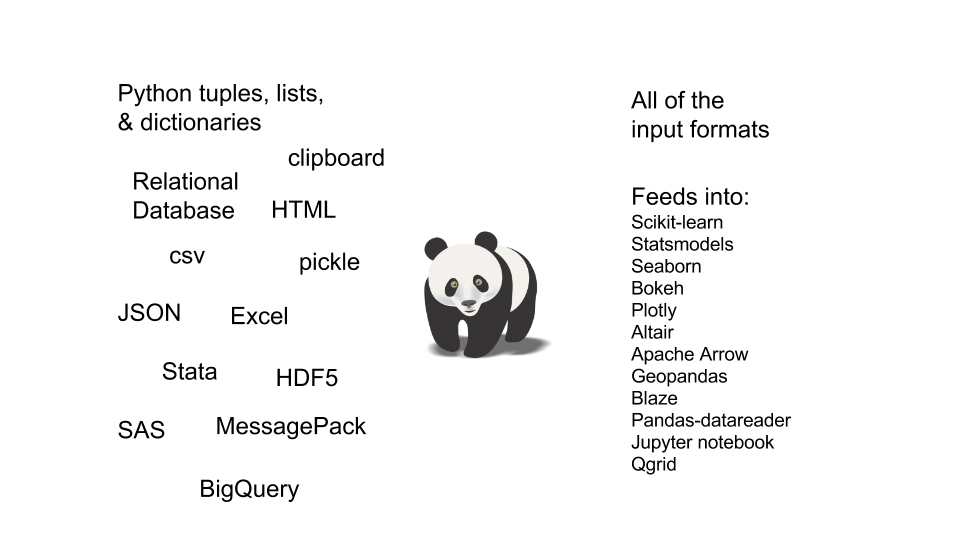
Pandas is good for:
- fast, repeatable data wrangling
- structured-ish data
- integration with Python data stack
- glue
Data Munging
Step 0: if you're new to Python, skip the yak shaving and download the Anaconda Python distribution.
- Get the data
- Explore
- Clean
- Augment & Prep
- Output
Step 1: Get The Data
Pandas makes it easy to create a DataFrame from existing data.
- Outlays (scroll down to Public Budget Database)
- "Deflators" (scroll down to Table 10.1)
In [57]:
# import things
import pandas as pd
import seaborn as sns
import matplotlib.pyplot as plt
import matplotlib
matplotlib.style.use('ggplot')
%matplotlib inline
pd.set_option('display.float_format', lambda x: '%.3f' % x)
In [58]:
# create a DataFrame from the outlays .csv
outlays = pd.read_csv('data/outlays.csv')
outlays.head()
Out[58]:
| Agency Code | Agency Name | Bureau Code | Bureau Name | Account Code | Account Name | Treasury Agency Code | Subfunction Code | Subfunction Title | BEA Category | ... | 2012 | 2013 | 2014 | 2015 | 2016 | 2017 | 2018 | 2019 | 2020 | 2021 | |
|---|---|---|---|---|---|---|---|---|---|---|---|---|---|---|---|---|---|---|---|---|---|
| 0 | 1 | Legislative Branch | 0 | Legislative Branch | nan | Receipts, Central fiscal operations | nan | 803 | Central fiscal operations | Mandatory | ... | 0 | 0 | 0 | 0 | 0 | 0 | 0 | 0 | 0 | 0 |
| 1 | 1 | Legislative Branch | 0 | Legislative Branch | nan | Receipts, Central fiscal operations | nan | 908 | Other interest | Net interest | ... | 0 | 0 | 0 | 0 | 0 | 0 | 0 | 0 | 0 | 0 |
| 2 | 1 | Legislative Branch | 0 | Legislative Branch | 241400.000 | Charges for services to trust funds | nan | 803 | Central fiscal operations | Mandatory | ... | 0 | 0 | 0 | 0 | 0 | 0 | 0 | 0 | 0 | 0 |
| 3 | 1 | Legislative Branch | 5 | Senate | 0.000 | Senate | 0.000 | 801 | Legislative functions | Discretionary | ... | 0 | 0 | 0 | 0 | 0 | 0 | 0 | 0 | 0 | 0 |
| 4 | 1 | Legislative Branch | 5 | Senate | 100.000 | Compensation of Members, Senate | 0.000 | 801 | Legislative functions | Mandatory | ... | 23,000 | 23,000 | 23,000 | 23,000 | 27,000 | 24,000 | 24,000 | 24,000 | 24,000 | 24,000 |
5 rows × 73 columns
In [59]:
# create a DataFrame from the "deflators" .xls  (requires xlrd library)
deflators = pd.read_excel('https://obamawhitehouse.archives.gov/sites/default/files/omb/budget/fy2017//assets/hist10z1.xls')
type(deflators)
Out[59]:
pandas.core.frame.DataFrame
In [60]:
outlays.tail()
Out[60]:
| Agency Code | Agency Name | Bureau Code | Bureau Name | Account Code | Account Name | Treasury Agency Code | Subfunction Code | Subfunction Title | BEA Category | ... | 2012 | 2013 | 2014 | 2015 | 2016 | 2017 | 2018 | 2019 | 2020 | 2021 | |
|---|---|---|---|---|---|---|---|---|---|---|---|---|---|---|---|---|---|---|---|---|---|
| 5081 | 902 | Undistributed Offsetting Receipts | 0 | Undistributed Offsetting Receipts | 977120.000 | Interest, Special Worker's Compensation Expenses | 16.000 | 902 | Interest received by on-budget trust funds | Net interest | ... | 0 | 0 | 0 | 0 | 0 | 0 | 0 | 0 | 0 | 0 |
| 5082 | 902 | Undistributed Offsetting Receipts | 0 | Undistributed Offsetting Receipts | 977910.000 | Employing agency contributions, Miscellaneous ... | 20.000 | 951 | Employer share, employee retirement (on-budget) | Mandatory | ... | 0 | 0 | 0 | 0 | 0 | 0 | 0 | 0 | 0 | 0 |
| 5083 | 902 | Undistributed Offsetting Receipts | 0 | Undistributed Offsetting Receipts | 977920.000 | Interest, Miscellaneous Trust Funds, Governmen... | 20.000 | 902 | Interest received by on-budget trust funds | Net interest | ... | 0 | 0 | 0 | 0 | 0 | 0 | 0 | 0 | 0 | 0 |
| 5084 | 902 | Undistributed Offsetting Receipts | 0 | Undistributed Offsetting Receipts | 997120.000 | Interest, Other DOD Trust Funds | 17.000 | 902 | Interest received by on-budget trust funds | Net interest | ... | 0 | 0 | 0 | 0 | -1,000 | -1,000 | -1,000 | -1,000 | -1,000 | -1,000 |
| 5085 | 930 | Miscellaneous Receipts Below the Reporting Thr... | 0 | Miscellaneous Receipts Below the Reporting Thr... | 901000.000 | Miscellaneous Unconverted Offsetting Receipts | 99.000 | 809 | Deductions for offsetting receipts | Mandatory | ... | -7,000 | 0 | -8,000 | -15,000 | 0 | 0 | 0 | 0 | 0 | 0 |
5 rows × 73 columns
In [61]:
# grab first 3 and the last 2 rows of the deflators dataframe

deflators.iloc[[0,1,2,-2,-1]]
Out[61]:
| Table 10.1—GROSS DOMESTIC PRODUCT AND DEFLATORS USED IN THE HISTORICAL TABLES: 1940–2021 | Unnamed: 1 | Unnamed: 2 | Unnamed: 3 | Unnamed: 4 | Unnamed: 5 | Unnamed: 6 | Unnamed: 7 | Unnamed: 8 | Unnamed: 9 | Unnamed: 10 | Unnamed: 11 | Unnamed: 12 | Unnamed: 13 | Unnamed: 14 | Unnamed: 15 | |
|---|---|---|---|---|---|---|---|---|---|---|---|---|---|---|---|---|
| 0 | (Fiscal Year 2009 = 1.000) | NaN | NaN | NaN | NaN | NaN | NaN | NaN | NaN | NaN | NaN | NaN | NaN | NaN | NaN | NaN |
| 1 | Fiscal Year | GDP (in billions of dollars) | GDP (Chained) Price Index | Composite Outlay Deflators | NaN | NaN | NaN | NaN | NaN | NaN | NaN | NaN | NaN | NaN | NaN | NaN |
| 2 | NaN | NaN | NaN | Total | Total Defense | Total Non- defense | Payment for Individuals | NaN | NaN | Other Grants | Net Interest | Undis- tributed Offsetting Receipts | All Other | Addendum: Direct Capital | NaN | NaN |
| 86 | 2021 estimate | 22875.200 | 1.229 | 1.255 | 1.236 | 1.258 | 1.258 | 1.258 | 1.259 | 1.361 | 1.229 | 1.283 | 1.259 | 1.198 | 1.193 | 1.214 |
| 87 | Note: Constant dollar research and development... | NaN | NaN | NaN | NaN | NaN | NaN | NaN | NaN | NaN | NaN | NaN | NaN | NaN | NaN | NaN |
Step 2: Explore
What kind of pain are you in for?
In [62]:
# see the column names
outlays.columns
Out[62]:
Index(['Agency Code', 'Agency Name', 'Bureau Code', 'Bureau Name',
       'Account Code', 'Account Name', 'Treasury Agency Code',
       'Subfunction Code', 'Subfunction Title', 'BEA Category',
       'Grant/non-grant split', 'On- or Off- Budget', '1962', '1963', '1964',
       '1965', '1966', '1967', '1968', '1969', '1970', '1971', '1972', '1973',
       '1974', '1975', '1976', 'TQ', '1977', '1978', '1979', '1980', '1981',
       '1982', '1983', '1984', '1985', '1986', '1987', '1988', '1989', '1990',
       '1991', '1992', '1993', '1994', '1995', '1996', '1997', '1998', '1999',
       '2000', '2001', '2002', '2003', '2004', '2005', '2006', '2007', '2008',
       '2009', '2010', '2011', '2012', '2013', '2014', '2015', '2016', '2017',
       '2018', '2019', '2020', '2021'],
      dtype='object')
In [63]:
# see datatypes and high-level view of missing data
# watch points:
# - is the number of rows in the ballpark?
# - are there codes coming in as numeric datatypes?
# - are there columns with unexpected null values?
# - are any of these column names going to be annoying?
# - NumPy loves floats! Are you planning to do any math?

outlays.info()
<class 'pandas.core.frame.DataFrame'>
RangeIndex: 5086 entries, 0 to 5085
Data columns (total 73 columns):
Agency Code              5086 non-null int64
Agency Name              5086 non-null object
Bureau Code              5086 non-null int64
Bureau Name              5086 non-null object
Account Code             5048 non-null float64
Account Name             5086 non-null object
Treasury Agency Code     4944 non-null float64
Subfunction Code         5086 non-null int64
Subfunction Title        5086 non-null object
BEA Category             5086 non-null object
Grant/non-grant split    5086 non-null object
On- or Off- Budget       5086 non-null object
1962                     5086 non-null object
1963                     5086 non-null object
1964                     5086 non-null object
1965                     5086 non-null object
1966                     5086 non-null object
1967                     5086 non-null object
1968                     5086 non-null object
1969                     5086 non-null object
1970                     5086 non-null object
1971                     5086 non-null object
1972                     5086 non-null object
1973                     5086 non-null object
1974                     5086 non-null object
1975                     5086 non-null object
1976                     5086 non-null object
TQ                       5086 non-null object
1977                     5086 non-null object
1978                     5086 non-null object
1979                     5086 non-null object
1980                     5086 non-null object
1981                     5086 non-null object
1982                     5086 non-null object
1983                     5086 non-null object
1984                     5086 non-null object
1985                     5086 non-null object
1986                     5086 non-null object
1987                     5086 non-null object
1988                     5086 non-null object
1989                     5086 non-null object
1990                     5086 non-null object
1991                     5086 non-null object
1992                     5086 non-null object
1993                     5086 non-null object
1994                     5086 non-null object
1995                     5086 non-null object
1996                     5086 non-null object
1997                     5086 non-null object
1998                     5086 non-null object
1999                     5086 non-null object
2000                     5086 non-null object
2001                     5086 non-null object
2002                     5086 non-null object
2003                     5086 non-null object
2004                     5086 non-null object
2005                     5086 non-null object
2006                     5086 non-null object
2007                     5086 non-null object
2008                     5086 non-null object
2009                     5086 non-null object
2010                     5086 non-null object
2011                     5086 non-null object
2012                     5086 non-null object
2013                     5086 non-null object
2014                     5086 non-null object
2015                     5086 non-null object
2016                     5086 non-null object
2017                     5086 non-null object
2018                     5086 non-null object
2019                     5086 non-null object
2020                     5086 non-null object
2021                     5086 non-null object
dtypes: float64(2), int64(3), object(68)
memory usage: 2.8+ MB
In [64]:
# math! note that our dollar amts aren't being treated as numeric values
outlays.describe()
Out[64]:
| Agency Code | Bureau Code | Account Code | Treasury Agency Code | Subfunction Code | |
|---|---|---|---|---|---|
| count | 5086.000 | 5086.000 | 5048.000 | 4944.000 | 5086.000 |
| mean | 106.277 | 19.283 | 166440.529 | 44.419 | 484.108 |
| std | 207.342 | 25.214 | 285555.505 | 32.740 | 249.309 |
| min | 1.000 | 0.000 | 0.000 | 0.000 | 51.000 |
| 25% | 9.000 | 0.000 | 566.000 | 14.000 | 302.000 |
| 50% | 15.000 | 9.000 | 4082.500 | 28.000 | 452.000 |
| 75% | 27.000 | 30.000 | 271715.000 | 75.000 | 751.000 |
| max | 930.000 | 99.000 | 997200.000 | 99.000 | 959.000 |
Step 2A: Get the Data Again
Yeah, you'll probably have to do that.
In [65]:
# some better data types
# - force selected columns to string/object
# - thousands parameter ensures incoming numbers w/ commas are not interpreted as string

outlays = pd.read_csv(
    'data/outlays.csv',
    thousands=',',
    dtype={'Agency Code': str,
           'Bureau Code': str,
           'Account Code': str,
           'Treasury Agency Code': str,
           'Subfunction Code': str}
    )
# dollar amounts now treated as numeric
outlays['1973'].describe()
Out[65]:
count       5086.000
mean       48310.506
std       924126.826
min     -8294670.000
25%            0.000
50%            0.000
75%            0.000
max     42955698.000
Name: 1973, dtype: float64
In [66]:
# take 2: deflators
# - only take the 1st 3 columns
# - specify better header names
# - ignore header rows in spreadsheet
# - ignore the footer row

deflators = pd.read_excel('data/hist10z1.xls',
                  parse_cols=2,
                  names=['fiscal_year', 'gdp_billions', 'deflator'],
                  header=None,
                  skiprows=5,
                  skip_footer=1
                 )
deflators.head()
Out[66]:
| fiscal_year | gdp_billions | deflator | |
|---|---|---|---|
| 0 | 1940 | 98.200 | 0.081 |
| 1 | 1941 | 116.200 | 0.084 |
| 2 | 1942 | 147.700 | 0.090 |
| 3 | 1943 | 184.600 | 0.096 |
| 4 | 1944 | 213.800 | 0.100 |
Step 3: Clean
The annoying stuff.
For example
- Renaming
- Handling missing values
- Delete unecessary data
- Clean up strings
- Tidy data
Clean up outlays
In [67]:
# Rename some columns

outlays = outlays.rename(columns = {
        'Agency Code': 'agency_code',
        'Agency Name': 'agency_name',
        'Bureau Code': 'bureau_code',
        'Bureau Name': 'bureau_name',
        'Account Code': 'account_code',
        'Account Name': 'account_name',
        'Treasury Agency Code': 'treasury_agency_code',
        'Subfunction Code': 'subfunction_code',
        'Subfunction Title': 'subfunction_name',
        'BEA Category': 'bea_category',
        'Grant/non-grant split': 'grant_split',
        'On- or Off- Budget': 'on_off_budget'
    })
outlays.columns
Out[67]:
Index(['agency_code', 'agency_name', 'bureau_code', 'bureau_name',
       'account_code', 'account_name', 'treasury_agency_code',
       'subfunction_code', 'subfunction_name', 'bea_category', 'grant_split',
       'on_off_budget', '1962', '1963', '1964', '1965', '1966', '1967', '1968',
       '1969', '1970', '1971', '1972', '1973', '1974', '1975', '1976', 'TQ',
       '1977', '1978', '1979', '1980', '1981', '1982', '1983', '1984', '1985',
       '1986', '1987', '1988', '1989', '1990', '1991', '1992', '1993', '1994',
       '1995', '1996', '1997', '1998', '1999', '2000', '2001', '2002', '2003',
       '2004', '2005', '2006', '2007', '2008', '2009', '2010', '2011', '2012',
       '2013', '2014', '2015', '2016', '2017', '2018', '2019', '2020', '2021'],
      dtype='object')
In [68]:
# Extraneous information

del outlays['TQ']
In [69]:
# Missing values

print(outlays[['account_code', 'treasury_agency_code', '2012']].head(2))
outlays = outlays.fillna({
        'account_code': 'missing',
        'treasury_agency_code': 'missing',
        '1962': 0 # not needed here, but included as an example
    })
print(outlays[['account_code', 'treasury_agency_code', '2012']].head(2))
  account_code treasury_agency_code  2012
0          NaN                  NaN     0
1          NaN                  NaN     0
  account_code treasury_agency_code  2012
0      missing              missing     0
1      missing              missing     0
In [70]:
# string clean-up
print(pd.unique(outlays.account_name.ravel()))
outlays.account_name = outlays.account_name.str.strip().str.lower()
print(pd.unique(outlays.account_name.ravel()))

# oops capitalize DOD again
outlays.account_name = outlays.account_name.str.replace(' dod ', ' DOD ') # regex works too
print(pd.unique(outlays.account_name.ravel()))

outlays.subfunction_title = outlays.account_name.str.strip().str.lower()
outlays.bea_category = outlays.bea_category.str.lower()
['Receipts, Central fiscal operations'
 'Charges for services to trust funds' 'Senate' ...,
 'Interest, Miscellaneous Trust Funds, Government-wide'
 'Interest, Other DOD Trust Funds'
 'Miscellaneous Unconverted Offsetting Receipts']
['receipts, central fiscal operations'
 'charges for services to trust funds' 'senate' ...,
 'interest, miscellaneous trust funds, government-wide'
 'interest, other dod trust funds'
 'miscellaneous unconverted offsetting receipts']
['receipts, central fiscal operations'
 'charges for services to trust funds' 'senate' ...,
 'interest, miscellaneous trust funds, government-wide'
 'interest, other DOD trust funds'
 'miscellaneous unconverted offsetting receipts']
In [71]:
# get discretionary spending only

disc = outlays[outlays['bea_category'] == 'discretionary']
# gut check number of rows
len(disc.index)
Out[71]:
2423
Clean up deflators
In [72]:
# clean up year column
# - get rid of the "estimate" text by applying a function to the fiscal_year Series

print(deflators.fiscal_year.unique())
deflators.fiscal_year = deflators.fiscal_year.map(lambda x: x[:4])
print('\n{}'.format(deflators.fiscal_year.unique()))
['1940' '1941' '1942' '1943' '1944' '1945' '1946' '1947' '1948' '1949'
 '1950' '1951' '1952' '1953' '1954' '1955' '1956' '1957' '1958' '1959'
 '1960' '1961' '1962' '1963' '1964' '1965' '1966' '1967' '1968' '1969'
 '1970' '1971' '1972' '1973' '1974' '1975' '1976' 'TQ' '1977' '1978' '1979'
 '1980' '1981' '1982' '1983' '1984' '1985' '1986' '1987' '1988' '1989'
 '1990' '1991' '1992' '1993' '1994' '1995' '1996' '1997' '1998' '1999'
 '2000' '2001' '2002' '2003' '2004' '2005' '2006' '2007' '2008' '2009'
 '2010' '2011' '2012' '2013' '2014' '2015' '2016 estimate' '2017 estimate'
 '2018 estimate' '2019 estimate' '2020 estimate' '2021 estimate']

['1940' '1941' '1942' '1943' '1944' '1945' '1946' '1947' '1948' '1949'
 '1950' '1951' '1952' '1953' '1954' '1955' '1956' '1957' '1958' '1959'
 '1960' '1961' '1962' '1963' '1964' '1965' '1966' '1967' '1968' '1969'
 '1970' '1971' '1972' '1973' '1974' '1975' '1976' 'TQ' '1977' '1978' '1979'
 '1980' '1981' '1982' '1983' '1984' '1985' '1986' '1987' '1988' '1989'
 '1990' '1991' '1992' '1993' '1994' '1995' '1996' '1997' '1998' '1999'
 '2000' '2001' '2002' '2003' '2004' '2005' '2006' '2007' '2008' '2009'
 '2010' '2011' '2012' '2013' '2014' '2015' '2016' '2017' '2018' '2019'
 '2020' '2021']
Step 3A: Tidy Data
Datasets are often constructed in bizarre ways
- Hadley Wickham, in his 2014 paper Tidy Data (Journal of Statistical Software, August 2014)
Principles of Tidy Data
- each variable is a column
- each observation is a row
- each type of observational unit is a table
- easy to model, manipulate, and visualize
In [73]:
# tidy the outlays (aka spending) dataset
# - variables = agency, bureau, account, year, subfunction, etc.
# - observation = dollar amount

# list of dataframe columns to use as identifier variables
# (all columns not listed will be unpivoted and added an additional identifier columm)
variables = ['agency_code', 'agency_name', 'bureau_code', 'bureau_name', 'account_code', 'account_name', 'treasury_agency_code', 'subfunction_code', 'subfunction_name', 'bea_category', 'grant_split', 'on_off_budget']
outlays = pd.melt(outlays,
               id_vars=variables,
               # name of the new, unpivoted identifier column
               var_name='fiscal_year',
               # name of the value column for the unpivoted data
               value_name='amount'
              )

outlays.head()
Out[73]:
| agency_code | agency_name | bureau_code | bureau_name | account_code | account_name | treasury_agency_code | subfunction_code | subfunction_name | bea_category | grant_split | on_off_budget | fiscal_year | amount | |
|---|---|---|---|---|---|---|---|---|---|---|---|---|---|---|
| 0 | 001 | Legislative Branch | 00 | Legislative Branch | missing | receipts, central fiscal operations | missing | 803 | Central fiscal operations | mandatory | Nongrant | On-budget | 1962 | -628 |
| 1 | 001 | Legislative Branch | 00 | Legislative Branch | missing | receipts, central fiscal operations | missing | 908 | Other interest | net interest | Nongrant | On-budget | 1962 | 0 |
| 2 | 001 | Legislative Branch | 00 | Legislative Branch | 241400 | charges for services to trust funds | missing | 803 | Central fiscal operations | mandatory | Nongrant | On-budget | 1962 | 0 |
| 3 | 001 | Legislative Branch | 05 | Senate | 0000 | senate | 00 | 801 | Legislative functions | discretionary | Nongrant | On-budget | 1962 | 26946 |
| 4 | 001 | Legislative Branch | 05 | Senate | 0100 | compensation of members, senate | 00 | 801 | Legislative functions | mandatory | Nongrant | On-budget | 1962 | 0 |
Useful Pandas Tidy-ing Functions
See also:
- Pandas docs: Reshaping and pivot tables
- Tidy Data in Python
Step 4: Fun Stuff
Calculating New Columns
We need inflation-adjusted amounts to look at spending trends over time.
In [74]:
# merge discretionary outlays and deflators dataframes
# - by default Pandas will use like column names as the merge key
# - this is very intuitive for SQL nerds

outlays = outlays.merge(deflators, how='left')
outlays.head()
Out[74]:
| agency_code | agency_name | bureau_code | bureau_name | account_code | account_name | treasury_agency_code | subfunction_code | subfunction_name | bea_category | grant_split | on_off_budget | fiscal_year | amount | gdp_billions | deflator | |
|---|---|---|---|---|---|---|---|---|---|---|---|---|---|---|---|---|
| 0 | 001 | Legislative Branch | 00 | Legislative Branch | missing | receipts, central fiscal operations | missing | 803 | Central fiscal operations | mandatory | Nongrant | On-budget | 1962 | -628 | 586.900 | 0.178 |
| 1 | 001 | Legislative Branch | 00 | Legislative Branch | missing | receipts, central fiscal operations | missing | 908 | Other interest | net interest | Nongrant | On-budget | 1962 | 0 | 586.900 | 0.178 |
| 2 | 001 | Legislative Branch | 00 | Legislative Branch | 241400 | charges for services to trust funds | missing | 803 | Central fiscal operations | mandatory | Nongrant | On-budget | 1962 | 0 | 586.900 | 0.178 |
| 3 | 001 | Legislative Branch | 05 | Senate | 0000 | senate | 00 | 801 | Legislative functions | discretionary | Nongrant | On-budget | 1962 | 26946 | 586.900 | 0.178 |
| 4 | 001 | Legislative Branch | 05 | Senate | 0100 | compensation of members, senate | 00 | 801 | Legislative functions | mandatory | Nongrant | On-budget | 1962 | 0 | 586.900 | 0.178 |
In [75]:
# Add calculated column to represent spending amount in 2009 dollars

outlays['amount_adj'] = outlays.amount / outlays.deflator
outlays[['fiscal_year', 'amount', 'amount_adj']].head()
Out[75]:
| fiscal_year | amount | amount_adj | |
|---|---|---|---|
| 0 | 1962 | -628 | -3522.154 |
| 1 | 1962 | 0 | 0.000 |
| 2 | 1962 | 0 | 0.000 |
| 3 | 1962 | 26946 | 151127.314 |
| 4 | 1962 | 0 | 0.000 |
Grouping
Summarize spending by category.
In [76]:
# get a list of budget function codes from sqlite & tweak to use as a lookup

from sqlalchemy import create_engine
db_engine = create_engine('sqlite:///data/pandas_data_munging.db')
functions = pd.read_sql_query(
    'SELECT budget_function_code, budget_function_desc FROM budget_function', db_engine
)

# index/sort the dataframe by budget_function_code
functions = functions.set_index(keys='budget_function_code').sort_index()
functions.head()
Out[76]:
| budget_function_desc | |
|---|---|
| budget_function_code | |
| 010 | national defense |
| 150 | international affairs |
| 250 | general science, space, and technology |
| 270 | energy |
| 300 | natural resources and environment |
In [77]:
# use the budget function information from sqllite to add this
# higher-level category to our discretionary spending dataframe
# (might not be the best approach but demos a few Pandas things)

def get_budget_function(sf):
    i = functions.index.get_loc(sf, method='ffill')
    return functions.iloc[i].budget_function_desc

subfunctions = pd.DataFrame(
    outlays.subfunction_code.unique(),
    columns=['subfunction_code']
)
subfunctions['function_name'] = subfunctions.subfunction_code.map(
    get_budget_function)
outlays = outlays.merge(subfunctions, how='left')
outlays[['subfunction_name', 'function_name']].tail()
Out[77]:
| subfunction_name | function_name | |
|---|---|---|
| 305155 | Interest received by on-budget trust funds | net interest |
| 305156 | Employer share, employee retirement (on-budget) | undistributed offsetting receipts |
| 305157 | Interest received by on-budget trust funds | net interest |
| 305158 | Interest received by on-budget trust funds | net interest |
| 305159 | Deductions for offsetting receipts | general government |
In [78]:
# group spending by year and category
grouped = outlays.groupby(['fiscal_year', 'function_name'])

grouped.agg({'amount_adj': 'sum'}).tail(10)
Out[78]:
| amount_adj | ||
|---|---|---|
| fiscal_year | function_name | |
| 2021 | income security | 482216528.388 |
| international affairs | 42545143.973 | |
| medicare | 610920774.361 | |
| national defense | 498161704.897 | |
| natural resources and environment | 37465430.291 | |
| net interest | 467040832.927 | |
| social security | 999925166.748 | |
| transportation | 105579144.298 | |
| undistributed offsetting receipts | -84646982.268 | |
| veterans benefits and services | 169685212.299 |
In [79]:
# use Seaborn library to plot a Pandas DataFrame
plot_df = outlays[['fiscal_year', 'function_name', 'amount_adj']]
plot_group = plot_df.groupby(['fiscal_year', 'function_name']).sum().reset_index()
sns.set(style="darkgrid")
ax = sns.tsplot(data=plot_group, time='fiscal_year', unit='function_name', value='amount_adj', err_style=None)

In [80]:
# group by years and calculate spending as % of GDP

by_year = outlays.groupby('fiscal_year')
def percent_gdp(group):
    spending = group['amount'] * 1000
    gdp = group['gdp_billions'] * 1000000000
    return spending.sum() / gdp.max() * 100

by_year.apply(percent_gdp)
Out[80]:
fiscal_year
1962   18.201
1963   17.974
1964   17.880
1965   16.635
1966   17.206
1967   18.786
1968   19.808
1969   18.695
1970   18.649
1971   18.777
1972   18.916
1973   18.120
1974   18.124
1975   20.634
1976   20.767
1977   20.174
1978   20.136
1979   19.612
1980   21.129
1981   21.611
1982   22.503
1983   22.828
1984   21.549
1985   22.161
1986   21.833
1987   20.996
1988   20.648
1989   20.534
1990   21.185
1991   21.673
1992   21.470
1993   20.742
1994   20.308
1995   19.988
1996   19.559
1997   18.874
1998   18.453
1999   17.894
2000   17.628
2001   17.633
2002   18.488
2003   19.060
2004   18.967
2005   19.179
2006   19.402
2007   19.051
2008   20.217
2009   24.404
2010   23.361
2011   23.428
2012   22.068
2013   20.940
2014   20.404
2015   20.717
2016   21.391
2017   21.485
2018   21.621
2019   22.102
2020   22.261
2021   22.401
dtype: float64
Useful tools:
- Applying operations over pandas DataFrames
- Pandas docs: apply-split-combine
- Pandas docs: computational tools (includes info on percent change, correlation, window functions)
- Pandas docs: time series/date functionality
Step 5: Output
In [81]:
# filter out the columns we don't want to write out
# (ran out of time to find a way to get rid of both columns in one line)
outlays_tidier = outlays.loc[:, outlays.columns != 'deflator']
outlays_tidier = outlays.loc[:, outlays.columns != 'gdp_billions']

# write to a .csv
outlays_tidier.to_csv('data/outlays_done.csv', index=False)
In [82]:
# dump to SQL db

db_engine = create_engine('sqlite:///data/pandas_data_munging.db')
outlays_tidier.to_sql(
    'outlays',
    db_engine,
    if_exists='replace',
    index=False
)
Resources
- Python for Data Analysis (by Wes McKinney): http://shop.oreilly.com/product/0636920023784.do
- Common Excel Tasks Demonstrated in Pandas: http://pbpython.com/excel-pandas-comp.html
- Pandas Cookbook: http://pandas.pydata.org/pandas-docs/stable/cookbook.html
- Useful Pandas Snippets: https://gist.github.com/bsweger/e5817488d161f37dcbd2
- Chris Albon's series of tutorials (scroll down to Data Wrangling)
- Pandas docs: how to do SQL operations in Pandas
- Giant panda image courtesy: http://www.clipartlord.com/2015/11/23/free-giant-panda-clip-art-3/