
Seeking the Invisible: Dark Matter Search with Neural Networks at ATLAS
Contents:
Dark Matter
Dark Matter at ATLAS
The ATLAS experiment
Running a Jupyter notebook
To setup everytime
Processes
Task 1: Can you print the 'DM_300' table?
Task 2: Estimate how many data points have lead_lep_pt below 100 GeV
Task 3: Estimate how many data points have lead_lep_pt between 100 and 150 GeV
Task 4: Estimate how many data points have lead_lep_pt above 500 GeV
Task 5: Estimate how many data points have lead_lep_pt below 150 GeV
Task 6: Estimate the average value of totalWeight in the DM_300 data
Task 7: Estimate how many Z+jets weighted events have lead_lep_pt below 125 GeV
Task 8: Estimate the maximum significance that can be achieved using lead_lep_pt
Task 9: Fill in the code to make a graph of 'sublead_lep_pt'
Task 10: Choose the x-values for your significance graph of 'sublead_lep_pt', then plot the significance graph
Task 11: Plot the significance for 'ETmiss', 'ETmiss_over_HT','dphi_pTll_ETmiss'
Intro to Machine Learning & Neural Networks
Build a Neural Network with your Mind!
After All, How do Machines Learn?
Neural Network variables
Training and Testing
Data Preprocessing
Task 12: Apply scaling transformations to X_test and X
Training the Neural Network model
Neural Network Output
Task 13: Plot the significance for 'NN_output'
Overtraining check
Universality Theorem
Going further
Dark Matter
Dark Matter is a hypothesised type of matter that does not interact with the electromagnetic force. It does not emit, absorb, or reflect light, making it invisible. So how has it been hypothesised? During various observations, astrophysicists have found that there isn't enough matter in space to account for all the gravitational attractions we measure! Therefore, there must be some invisible matter interacting with visible matter through Gravity.
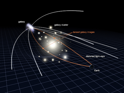
Let's look at one example quickly: gravitational lensing. It is when light gets bent around objects in space due to the gravitational fields around massive bodies. This lets you see behind objects in space!
| Diagram | Picture |
|---|---|
 |
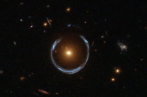 |
We see that mass has an effect on the path that light travels, so how does this relate to dark matter? Astrophysicists have seen light from distant objects that have been gravitationally lensed 'too much' - with the amount of observable mass causing the lensing, they should not see some objects that they in fact do! This then implies that there must be some more mass there that we can't see - dark matter!
Got interested and want to know more? Check this talk on “How the ATLAS experiment searches for Dark Matter” by Dr Christian Ohm (to be watched from the timestamp set in the link).
The ATLAS experiment
The ATLAS experiment is a collaboration between thousands of scientists and engineers across the world to maintain the operation of the ATLAS detector and analyse the data it records to try and find new particles. Just like we are going to do!

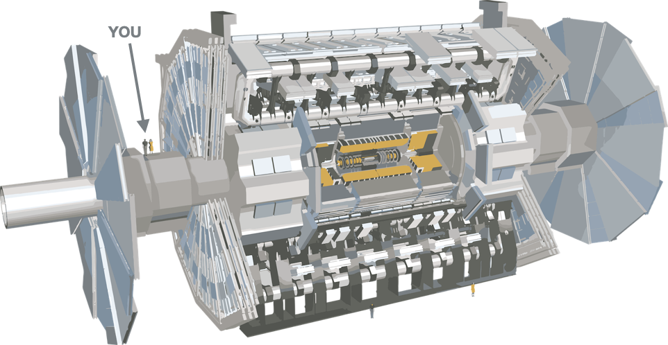
The ATLAS detector is a general-purpose particle detector used to detect the particles that come out of the collisions of the Large Hadron Collider (LHC). It is a massive 46 metres long and 25 metres in diameter! You can explore a 3D model of the detector here and learn more about its different parts and tools here.
| ATLAS vs Person | ATLAS vs Bus |
|---|---|
 |
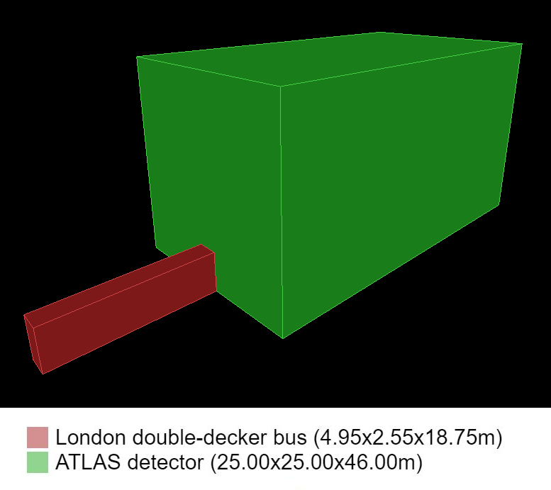 |
Want to know more?
- Link to an animation series that describes and explains the ATLAS detector (by CERN).
- Link to a more informal introduction to the ATLAS detector (by Sixty Symbols).
Dark Matter at ATLAS
So if dark matter is so common across the universe and its effects are clearly observed by astrophysicists, it should be easy to create and observe it using the ATLAS detector, right?
Unfortunately, not. Because we can't directly observe dark matter, there are many hypotheses of what it actually is. One hypothesis, or model, that we will be searching for is called a Weakly Interacting Massive Particle (WIMP).
As you can guess from the name, this type of dark matter particle is hard to detect because it doesn't really interact with other things. For example WIMPs don't interact with electromagnetic radiation, including light. Hence, we can't see them!
So what can we do to detect dark matter? Well if we can't see the dark matter around us, let's make the dark matter ourselves and see what happens!
At the LHC we collide particles together and look at new particles that are created from these collisions. What we can do is collide protons and look to see if any of those collisions produce dark matter particles! In the next section, we'll specifically look at the hypothesised process that creates dark matter.
Running a Jupyter notebook
You can run a single code cell by clicking on it then pressing Shift+Enter on your keyboard.
To setup everytime
to be run every time you re-open this notebook
We're going to be using a number of tools to help us:
- pandas: lets us store data as dataframes, a format widely used in Machine Learning
- numpy: provides numerical calculations such as histogramming
- matplotlib: common tool for making plots, figures, images, visualisations
import pandas # to store data as dataframe
import numpy # for numerical calculations such as histogramming
import matplotlib.pyplot # for plotting
Processes
The Dark Matter process we'll be looking for is 'DM_300', which we call "signal". The others are processes that may look like our signal, so we have to consider them as well, which we call "backgrounds".
processes = ['Non-resonant_ll','Z+jets','WZ','ZZ','DM_300']
This is where the data files are read
data_all = {} # dictionary to hold all data
for s in processes: # loop over different processes
    print(s)
    data_all[s] = pandas.read_csv('https://atlas-opendata.web.cern.ch/atlas-opendata/samples/2020/csv/DM_ML_notebook/'+s+'.csv') # read data files
Let's take a look at the data for the 'ZZ' process.
data_all['ZZ']
Task 1: Can you print the 'DM_300' table?
# your code for Task 1 here
Click me for Hint 1
All you need to do compared to data_all['ZZ'] above is change ZZ to DM_300
Click me for Solution 1
data_all['DM_300']
The dataset for each process is like a table of values. Each row is a different particle collision (what we call event). Each column is a different variable measured in that particle collision.
Let's make some graphs of the different variables in our datasets.
First, the leading lepton $p_T$ ('lead_lep_pt')
Let's first look at the 'lead_lep_pt' column of the 'DM_300' data table.
data_all['DM_300']['lead_lep_pt']
Now let's plot this in a histogram.
matplotlib.pyplot.hist(data_all['DM_300']['lead_lep_pt'])
It's always a good idea to add an x-axis label to your graph.
matplotlib.pyplot.hist(data_all['DM_300']['lead_lep_pt'])
matplotlib.pyplot.xlabel('lead_lep_pt') # x-axis label
...and x-axis units!
matplotlib.pyplot.hist(data_all['DM_300']['lead_lep_pt'])
matplotlib.pyplot.xlabel('lead_lep_pt [GeV]') # x-axis label
...and a y-axis label.
matplotlib.pyplot.hist(data_all['DM_300']['lead_lep_pt'])
matplotlib.pyplot.xlabel('lead_lep_pt [GeV]') # x-axis label
matplotlib.pyplot.ylabel('Events') # y-axis label
It's also a good idea to add a label and a legend to a graph.
matplotlib.pyplot.hist(data_all['DM_300']['lead_lep_pt'], label='DM')
matplotlib.pyplot.xlabel('lead_lep_pt [GeV]') # x-axis label
matplotlib.pyplot.ylabel('Events') # y-axis label
matplotlib.pyplot.legend() # add legend to plot
Task 2: Estimate by eye from the graph above how many events have lead_lep_pt below 100 GeV.
Click me for Hint 2
On the x-axis there's 1 bar below 100. Read across from the top of that bar to the y-axis to get the number of events.
Click me for Solution 2
About 190
Task 3: Estimate by eye from the graph above how many events have lead_lep_pt between 100 and 150 GeV.
Click me for Hint 3
On the x-axis there's 1 bar between 100 and 150. Read across from the top of that bar to the y-axis to get the number of data points.
Click me for Solution 3
About 175
Task 4: Estimate by eye from the graph above how many data points have lead_lep_pt above 500 GeV.
Click me for Hint 4
On the x-axis there's 1 bar above 500. Read across from the top of that bar to the y-axis to get the number of events.
Click me for Solution 4
1? Maybe 2? Not many that's for sure!
Task 5: Estimate by eye from the graph above how many data points have lead_lep_pt below 150 GeV.
Click me for Hint 5
On the x-axis there are 2 bars below 150. Read across from the top of those bars to the y-axis to get the number of events for each. Add those two numbers together.
Click me for Solution 5
About 190+175=365
We need to scale the graph using the 'totalWeight' column to get the number of collisions that would actually be measured, as opposed to the number of collisions that were generated by our computer simulations.
matplotlib.pyplot.hist(data_all['DM_300']['lead_lep_pt'], weights=data_all['DM_300']['totalWeight'], label='DM')
matplotlib.pyplot.xlabel('lead_lep_pt [GeV]') # x-axis label
matplotlib.pyplot.ylabel('Weighted Events') # y-axis label
matplotlib.pyplot.legend() # add legend to plot
Task 6: Comparing the above graph without weighting and the graph with weighting, estimate by eye the average value of totalWeight in the DM_300 data.
You can also use python as a calculator like:
342/4356
Click me for Hint 6
You could divide the number of weighted events in the first bar by the number of events in the first bar to get an estimate.
Click me for Solution 6
About 12.2/190 = 0.064
Now we need to stack the processes on top of each other in the graph. To do this, we for loop over the different processes.
stacked_variable = [] # list to hold variable to stack
stacked_weight = [] # list to hold weights to stack
for s in processes: # loop over different processes
    stacked_variable.append(data_all[s]['lead_lep_pt']) # get each value of variables
    stacked_weight.append(data_all[s]['totalWeight']) # get each value of weight
matplotlib.pyplot.hist(stacked_variable, weights=stacked_weight, label=processes, stacked=True)
matplotlib.pyplot.xlabel('lead_lep_pt [GeV]') # x-axis label
matplotlib.pyplot.ylabel('Weighted Events') # y-axis label
matplotlib.pyplot.legend() # add legend to plot
Task 7: Estimate by eye from the graph above how many Z+jets weighted events have lead_lep_pt below 125 GeV.
Click me for Hint 7
On the x-axis, there's 1 bar below about 125 GeV. Read across to the y-axis from the top of the Z+jets. Read across to the y-axis from the bottom of the Z+jets. Subtract those two numbers.
Click me for Solution 7
About 130-80=50
In particle physics, we declare that we have evidence for a process such as Dark Matter if we find a "significance" over 3.
significance = $\frac{\text{total signal weights}}{\sqrt{\text{total background weights}}}$
So let's see what significances we get for different variables. Can we get above 3?
x_values = [25,50,75,100,125,150,175,200] # the x-values at which significance will be calculated
# Taking a look at the graph above, the maximum x-value at which there's a mix of
# different colours present is a bit over 200.
# So we wrote the x-values up to 200 in gaps of 25.
# If you want, you can try different x-values later and see how it looks.

sigs = [] # list to hold significance values
for x in x_values: # loop over bins
    signal_weights_selected = 0 # start counter for signal weights
    background_weights_selected = 0 # start counter for background weights
    for s in processes: # loop over background samples
        if 'DM' in s: signal_weights_selected += sum(data_all[s][data_all[s]['lead_lep_pt']>x]['totalWeight'])
        else: background_weights_selected += sum(data_all[s][data_all[s]['lead_lep_pt']>x]['totalWeight'])
    sig_value = signal_weights_selected/numpy.sqrt(background_weights_selected)
    sigs.append(sig_value) # append to list of significance values

matplotlib.pyplot.plot( x_values[:len(sigs)], sigs ) # plot the data points
matplotlib.pyplot.ylabel('Significance') # y-axis label
Task 8: Estimate by eye from the graph above the maximum significance that can be achieved using lead_lep_pt.
Click me for Hint 8
Read across to the y-axis from the highest point on the graph.
Click me for Solution 8
About 2.53
Not the significance over 3 we were hoping for :(
What about any other variables?
Task 9: Fill in the code to make a graph of 'sublead_lep_pt'
stacked_variable = [] # list to hold variable to stack
stacked_weight = [] # list to hold weights to stack
for s in processes: # loop over different processes
    stacked_variable.append(data_all[s]['...']) # get each value of variables
    stacked_weight.append(data_all[s]['totalWeight']) # get each value of weight
matplotlib.pyplot.hist(stacked_variable, weights=stacked_weight, label=processes, stacked=True)
matplotlib.pyplot.xlabel('... [GeV]') # x-axis label
matplotlib.pyplot.ylabel('Weighted Events') # y-axis label
matplotlib.pyplot.legend() # add legend to plot
Click me for Hint 9
All you need to do compared to the colourful graph above is change the red text from 'lead_lep_pt' to 'sublead_lep_pt'
Click me for Solution 9
stacked_variable = [] # list to hold variable to stack
stacked_weight = [] # list to hold weights to stack
for s in processes: # loop over different processes
    stacked_variable.append(data_all[s]['sublead_lep_pt']) # get each value of variable
    stacked_weight.append(data_all[s]['totalWeight']) # get each value of weight
matplotlib.pyplot.hist(stacked_variable, weights=stacked_weight, label=processes, stacked=True)
matplotlib.pyplot.xlabel('sublead_lep_pt [GeV]') # x-axis label
matplotlib.pyplot.ylabel('Weighted Events') # y-axis label
matplotlib.pyplot.legend() # add legend to plot
Task 10: Choose the x-values for your significance graph of 'sublead_lep_pt', then plot the significance graph
There isn't really "correct" answer for the x-values, just something that shows the significance across a range of values.
Only click on the hints if you need.
x_values = [...your job to fill...] # the x-values at which significance will be calculated

sigs = [] # list to hold significance values
for x in x_values: # loop over bins
    signal_weights_selected = 0 # start counter for signal weights
    background_weights_selected = 0 # start counter for background weights
    for s in processes: # loop over background samples
        if 'DM' in s: signal_weights_selected += sum(data_all[s][data_all[s]['...']>x]['totalWeight'])
        else: background_weights_selected += sum(data_all[s][data_all[s]['...']>x]['totalWeight'])
    sig_value = signal_weights_selected/numpy.sqrt(background_weights_selected)
    sigs.append(sig_value) # append to list of significance values

matplotlib.pyplot.plot( x_values[:len(sigs)], sigs ) # plot the data points
matplotlib.pyplot.ylabel('Significance') # y-axis label
Click me for Hint 10.1
What's the maximum x-value at which there's a mix of different colours present in the 'sublead_lep_pt' graph?
Click me for Hint 10.2
Compared to the code for the significance graph above, you only need to change the red text from 'lead_lep_pt' to 'sublead_lep_pt'
Click me for Solution 10
x_values = [15,30,45,60,75,90,105,120,135,150] # the x-values for significance

sigs = [] # list to hold significance values
for x in x_values: # loop over bins
    signal_weights_selected = 0 # start counter for signal weights
    background_weights_selected = 0 # start counter for background weights
    for s in processes: # loop over background samples
        if 'DM' in s: signal_weights_selected += sum(data_all[s][data_all[s]['lead_lep_pt']>x]['totalWeight'])
        else: background_weights_selected += sum(data_all[s][data_all[s]['lead_lep_pt']>x]['totalWeight'])
    sig_value = signal_weights_selected/numpy.sqrt(background_weights_selected)
    sigs.append(sig_value) # append to list of significance values

matplotlib.pyplot.plot( x_values[:len(sigs)], sigs ) # plot the data points
matplotlib.pyplot.ylabel('Significance') # y-axis label
Can we get a significance above 3 for 'sublead_lep_pt'?
What about any other variables?
Task 11: Plot the significance for 'ETmiss', 'ETmiss_over_HT','dphi_pTll_ETmiss'.
'ETmiss' has units [GeV], 'ETmiss_over_HT' has no units and 'dphi_pTll_ETmiss' has units [rad]
# your code for Task 3 here
Click me for part 1 to Solution 11
stacked_variable = [] # list to hold variable to stack
stacked_weight = [] # list to hold weights to stack
for s in processes: # loop over different processes
    stacked_variable.append(data_all[s]['ETmiss']) # get each value of variable
    stacked_weight.append(data_all[s]['totalWeight']) # get each value of weight
matplotlib.pyplot.hist(stacked_variable, weights=stacked_weight, label=processes, stacked=True)
matplotlib.pyplot.xlabel('ETmiss [GeV]') # x-axis label
matplotlib.pyplot.ylabel('Weighted Events') # y-axis label
matplotlib.pyplot.legend() # add legend to plot
Click me for part 2 to Solution 11
x_values = [100,150,200,250,300,350,400,450,500] # the x-values for significance

sigs = [] # list to hold significance values
for x in x_values: # loop over bins
    signal_weights_selected = 0 # start counter for signal weights
    background_weights_selected = 0 # start counter for background weights
    for s in processes: # loop over background samples
        if 'DM' in s: signal_weights_selected += sum(data_all[s][data_all[s]['ETmiss']>x]['totalWeight'])
        else: background_weights_selected += sum(data_all[s][data_all[s]['ETmiss']>x]['totalWeight'])
    sig_value = signal_weights_selected/numpy.sqrt(background_weights_selected)
    sigs.append(sig_value) # append to list of significance values

matplotlib.pyplot.plot( x_values[:len(sigs)], sigs ) # plot the data points
matplotlib.pyplot.ylabel('Significance') # y-axis label
Click me for part 3 to Solution 11
stacked_variable = [] # list to hold variable to stack
stacked_weight = [] # list to hold weights to stack
for s in processes: # loop over different processes
    stacked_variable.append(data_all[s]['ETmiss_over_HT']) # get each value of variable
    stacked_weight.append(data_all[s]['totalWeight']) # get each value of weight
matplotlib.pyplot.hist(stacked_variable, weights=stacked_weight, label=processes, stacked=True)
matplotlib.pyplot.xlabel('ETmiss_over_HT') # x-axis label
matplotlib.pyplot.ylabel('Weighted Events') # y-axis label
matplotlib.pyplot.legend() # add legend to plot
Click me for part 4 to Solution 11
x_values = [0.5,0.6,0.7,0.8,0.9,1.0,1.1,1.2] # the x-values at for significance

sigs = [] # list to hold significance values
for x in x_values: # loop over bins
    signal_weights_selected = 0 # start counter for signal weights
    background_weights_selected = 0 # start counter for background weights
    for s in processes: # loop over background samples
        if 'DM' in s: signal_weights_selected += sum(data_all[s][data_all[s]['ETmiss_over_HT']>x]['totalWeight'])
        else: background_weights_selected += sum(data_all[s][data_all[s]['ETmiss_over_HT']>x]['totalWeight'])
    sig_value = signal_weights_selected/numpy.sqrt(background_weights_selected)
    sigs.append(sig_value) # append to list of significance values

matplotlib.pyplot.plot( x_values[:len(sigs)], sigs ) # plot the data points
matplotlib.pyplot.ylabel('Significance') # y-axis label
Click me for part 5 to Solution 11
stacked_variable = [] # list to hold variable to stack
stacked_weight = [] # list to hold weights to stack
for s in processes: # loop over different processes
    stacked_variable.append(data_all[s]['dphi_pTll_ETmiss']) # get each value of variables
    stacked_weight.append(data_all[s]['totalWeight']) # get each value of weight
matplotlib.pyplot.hist(stacked_variable, weights=stacked_weight, label=processes, stacked=True)
matplotlib.pyplot.xlabel('dphi_pTll_ETmiss [rad]') # x-axis label
matplotlib.pyplot.ylabel('Weighted Events') # y-axis label
matplotlib.pyplot.legend() # add legend to plot
Click me for part 6 to Solution 11
x_values = [2,2.1,2.2,2.3,2.4,2.5,2.6,2.7,2.8,2.9,3.0] # the x-values for significance

sigs = [] # list to hold significance values
for x in x_values: # loop over bins
    signal_weights_selected = 0 # start counter for signal weights
    background_weights_selected = 0 # start counter for background weights
    for s in processes: # loop over background samples
        if 'DM' in s: signal_weights_selected += sum(data_all[s][data_all[s]['dphi_pTll_ETmiss']>x]['totalWeight'])
        else: background_weights_selected += sum(data_all[s][data_all[s]['dphi_pTll_ETmiss']>x]['totalWeight'])
    sig_value = signal_weights_selected/numpy.sqrt(background_weights_selected)
    sigs.append(sig_value) # append to list of signifcance values

matplotlib.pyplot.plot( x_values[:len(sigs)], sigs ) # plot the data points
matplotlib.pyplot.ylabel('Significance') # y-axis label
If no single variable can get significance above 3, what else can we do?
Introduction to Machine Learning and Neural Networks
Neural networks (NN) are not your typical computer program. They are part of a broad group of algorithms that use Machine Learning (ML). While the conventional idea of a computer program is a precise set of instructions for a computer to follow, Machine Learning allows the computer to achieve goals it was not specifically instructed to perform. From a general set of principles, ML grants computers a wide range of applications.
A more formal definition of a Machine Learning algorithm is something along the lines of: a program for automated analytical modelling. Let’s dissect each term of this description using neural networks as an example. At first, the network takes a set of inputs from a dataset we want to know more about (analytical). It then makes decisions to optimize its success in analysing these inputs (automated). Finally, it gives an output that highlights patterns found in the dataset (modelling). The type of data the neural network receives and its structure are defined by the programmer, you. But once all parameters are set, the program will perform tasks without requiring explicit, line by line, instructions on how to do them!
As you may have noticed, we are going to focus on neural networks for this workbook since it is one of the most widely used computational techniques. In essence, NNs can be understood as functions. Just like y=ax+b, they require an input (x) to interact with some inner parameters (a and b) so that an output (y) can be produced. In this sense, neural networks attempt to solve a specific task by modelling a function that may or not be similar to a conventional computer program that was instructed to solve the same thing. The reality is that neural networks can have up to several thousands of inner parameters, making things more complex. Although a slightly more in-depth discussion of this matter can be found in the section “The Universality Theorem”, let’s stick to an analogy for now.
Build a Neural Network with your Mind!
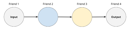
In this section, we will use a thought experiment to understand the structure and functioning of neural networks. To break the silence, a group of friends decide to play a certain game. The goal of this game is to accurately identify images of cats and dogs. We shall refer to these two categories as classes because they can be distinguished upon evaluating their characteristics. Each individual characteristic such as number of paws or weight is referred to as a descriptor since it describes the animal. To make the game challenging, no player can single-handedly guess the class. Instead, the players have to form some sort of assembly line that begins with raw materials (descriptors) and ends with a product (classification). Also similarly, each player can only receive information from their previous neighbor and send information to their next neighbor. For a group of four friends, the network structure might look something like the diagram below.
Amongst many approaches to this game, the friends decide to transform the descriptors from Friend 1 into a sentence that Friend 4 will easily be able to interpret as either a cat or a dog. Following the assembly line: Friend 1 looks at an image and notes down a characteristic of the animal; Friend 2 gets the descriptor and converts it into an adjective; Friend 3 receives the adjective and writes a description from it; Friend 4 then finally reads the description and yells the class of the animal. If Friend 1 verifies that Friend 4 is correct, they won the game. Else, they lost the round. Therefore, the success of the goal depends on the independent reasoning of each neuron as well as collaboration via a collection of processed information. With the plan set, the group of friends decide to give it a try, here using “height” as the descriptor (see diagram below).
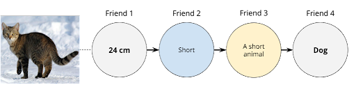
As we can observe, Friend 4 had no clue whether the animal was a cat or a dog. For all Friend 4 is concerned, deciding between a cat or a dog is a fifty-fifty probability scenario akin to tossing a coin to give an answer. The issue lies in the fact that both animals share common features such as having four legs, whiskers, and tails. In the previous round, a short animal could be both a normal-sized cat or a small-sized dog like a Welsh Corgi or a Chihuahua. Hence, it becomes hard to distinguish between them with only one descriptor. For this reason, a better approach is to increase the number of initial friends, or inputs, we have in our game to something like the diagram below. Notice how we now have a layer of friends to perform the same task, in this case, to evaluate one descriptor each.

In more technical terms, each friend represents a neuron of a neural network. The design and functioning of these neurons were inspired by biological neurons but should not be treated as such. Complementing the discussion in the previous section, the neurons are the ones that hold the inner parameters of a network. Any optimization then requires the tweaking of these individual parameters.
Back to our thought-experiment, the group of friends decides to call two more players to the game. By forming a layer with Friend 1, these two extra friends will allow the group to input two more descriptors. In the upcoming diagrams, the group decides to use the following inputs: height as Input A; whisker length as Input B, and fur pattern as Input C. Each friend in Friend Layer 1 can only evaluate one descriptor from the image. While each friend still performs the same tasks, the group hopes to get better results this time. Two example outcomes can be seen in the diagrams below.
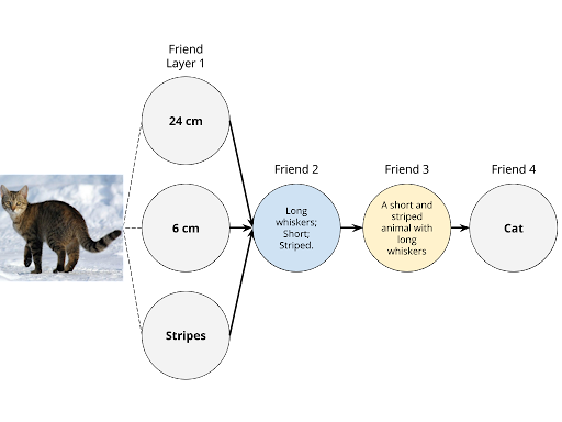

Gladly, we see Friend 4 outputs the correct classification of the image even though only Friend Layer 1 had access to the original image. Most importantly, there is an increasing degree of pattern recognition along the network of friends that allows each friend to perform optimally to accurately classify cats and dogs.
data_NN = {} # define empty dictionary to hold dataframes that will be used to train the NN

NN_inputs = [
             #'sum_lep_charge',
             'lead_lep_pt',
             'sublead_lep_pt',
             'mll',
             'ETmiss',
             #'dRll',
             'dphi_pTll_ETmiss',
             'fractional_pT_difference',
             'ETmiss_over_HT',
             #'N_bjets'
            ] # list of variables for Neural Network

for s in processes: # loop over the different processes
    data_NN[s] = data_all[s][NN_inputs].copy() # copy variables into data for NN
The type of ML algorithm that accomplishes classification is called a Machine Learning classifier. Although there are other types of ML models that accomplish other goals, classifiers are widely used in HEP. More specifically, binary classifiers are used to distinguish signal from background for particle collision events detected by instruments such as ATLAS. In fact, this is an endeavour you have already explored and attempted to optimize by choosing selection cuts. Hence, we shall focus solely on ML classifiers for this course.
Organise data ready for the NN
# for NNs data is usually organised
# into one 2D array of shape (n_samples x n_features)
# containing all the data and one array of categories
# of length n_samples

all_processes = [] # define empty list that will contain all features for the MC
for s in processes: # loop over the different keys in the dictionary of dataframes
    all_processes.append(data_NN[s]) # append the MC dataframe to the list containing all MC features
X = numpy.concatenate(all_processes) # merge the list of MC dataframes into a single 2D array of features, called X

all_y = [] # define empty list that will contain labels whether an event in signal or background
for s in processes: # loop over the different keys in the dictionary of dataframes
    if 'DM' in s: # only signal MC should pass this
        all_y.append(numpy.ones(data_NN[s].shape[0])) # signal events are labelled with one
    else: # background if gets here
        all_y.append(numpy.zeros(data_NN[s].shape[0])) # background events are labelled with zero
y = numpy.concatenate(all_y) # merge the list of labels into a single 1D array of labels, called y
The above analogy can be generalized into an algorithm for the classification of audio files, text, numerical sequences, and any other data that can be separated into a set of distinguishable classes. But what are the advantages of using neural networks instead of having a human do the analysis? Unfortunately, the answer is not that straight-forward. Yet, two arguments give a significant advantage to neural networks.
In contrast with our thought-experiments, real-life resources are scarce and we must take them into consideration when analysing data. For any task performed, computational resources are needed. Anything from electricity, hardware, to time spent between input and output are taken as computational resources. The overall consumption of these resources is called computational cost. And, we can use this cost to compare the efficiency of techniques and choose the best one for our goal.
So what are the arguments? Firstly, iterating over huge datasets recorded at ATLAS requires a great amount of computational resources. While humans spend a lot of time and energy, neural networks are designed to be efficient at repeatability. Hence, NNs offer a significantly lower computational cost than manual analysis when iterating over thousands of events. Secondly, NNs can achieve a higher degree of optimization than manual selection cuts and often even go beyond the humanly obvious to find correlations between data points that increase the accuracy of classification. The caveat is that these are black box algorithms. They are not completely transparent, which makes their decision-making process inaccessible. To continue our journey, we must now ponder: how do machines even learn?
After All, How do Machines Learn?
Before we begin, we first need to plan how the teaching will unfold. And that is up to us to decide. What a responsibility! Gladly, a few concepts in neural networks are commonly used across multiple fields. By knowing these fundamentals, we can begin to tackle a wide range of analytical problems.
Imagine that you are hiking in a foggy mountainscape. You got tired and now want to get down the valley where all close-by cities are located. As you descend to higher pressure levels, the fog increases and the range of your field of view consequently decreases. To avoid any potential obstacles or dangerous pitfalls, you stop and carefully scout the terrain as far down as your field of view can reach. Hence, the distance you cover between stepping and scouting reduces as your field of view decreases in range. However, this slower pace is a good indicator since it implies you are getting closer to the city! Essentially, you are guided to lower your altitude by the decrease in the distance covered per interval of stepping and scouting. You might not reach a city at sea-level (e.g. Stockholm) but you surely will achieve your goal of finding a city in a valley (e.g. Zermatt).

Similarly to how you hiked an imaginary mountainscape by following the fog, a neural network finds a local minima (valley) of a function through a gradient descent. This function should not be confused with the neural network function we discussed in the previous section. It numerically evaluates the overall performance of the modelled neural network function in accomplishing classification. High values of the function indicate a poor performance whereas low values, a good one. Therefore, we call it the loss function. Back to our analogy, the loss function can be thought of as the shape of the terrain and its values as the hiker’s altitude, which tells us how far down we still have to go. The number of axes (dimensions) of this function is equal to the number of inputs it takes. For example, our cats and dogs classifier from the previous section has a 3-dimensional loss function since it takes three different descriptors.
Following the same logic, gradient descent is analogous to the whole process of hiking down the mountain and it is related to the steepness of the loss function. In more technical terms, it is the iterative process of calculating the current value of the loss function (scouting) and then altering the inner parameters of the NN by a step down in the loss function (stepping). The NN repeats this process through multiple iterations, each time decreasing the step size (field of view decreases) until it reaches a model optimized for successfully classifying signal and background events (a city is reached).
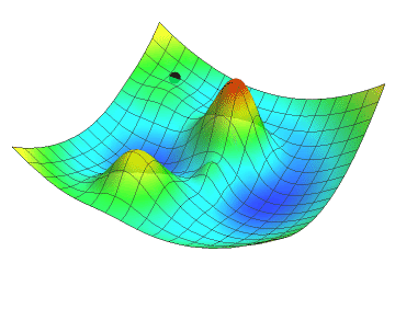
In the animation below, the black dot represents the position of a neural network as it descends along the gradient by a definite step size. Just like you might see in a topographic map, the gradient of the loss function is colour-coded in a mesh where red are the peaks and blue are the valleys. Note how the descent slows down as the gradient flattens. Did your hiking adventure look like that?
No matter which goal a neural network is developed to achieve, the learning process will inherently use concepts such as the loss function and gradient descent. Although we did not go into the details about the inner parameters of neural networks, let’s get hands-on and start coding!
Training and testing
Isn’t it the dream of every student to get very similar exam questions to ones they practiced with? It is easy to score well when you are familiarized with the problems being asked. To guarantee a fair test, teachers make sure to split their bank of questions into a training and a testing set. As such, students will have plenty to practice but still receive unseen questions on the test. The same applies to neural networks!
Before running the algorithm, we must first split the input data into the two sets: training and testing. Furthermore, this separation has to be randomized to avoid selection bias (just like when cutting a deck of cards). Now, let’s see how this process is coded.
from sklearn.model_selection import train_test_split

# make train and test sets
X_train,X_test,y_train,y_test = train_test_split(X, y)
Data Preprocessing for Neural Network
A Neural Network may have difficulty converging if the data is not standardised. Note that you must apply the same standardisation to the test set for meaningful results.
from sklearn.preprocessing import StandardScaler
scaler = StandardScaler() # initialise StandardScaler

# Fit only to the training data
scaler.fit(X_train)

# Now apply the transformations to the data:
X_train = scaler.transform(X_train)
Task 12: Apply the same transformations to X_test and X
# your code for Task 4 here
Click me for Hint 12
Copy and paste the line X_train = scaler.transform(X_train) into a code cell, but change X_train to X_test
Click me for Solution 12
X_test = scaler.transform(X_test)
X = scaler.transform(X)
from sklearn.neural_network import MLPClassifier

ml_classifier = MLPClassifier( ) # create instance of the model

ml_classifier.fit(X_train,y_train) # Now we can fit the training data to our model
Neural Network Output
Here we get the Neural Network's output for every event (so could be signal, background...). The higher the output, the more the Neural Network thinks that event looks like signal.
y_predicted = ml_classifier.predict_proba(X)[:, 1]
In this cell we save the Neural Network output to our dataframes.
cumulative_events = 0 # start counter for total number of events for which output is saved
for s in processes: # loop over samples
    data_all[s]['NN_output'] = y_predicted[cumulative_events:cumulative_events+len(data_all[s])]
    cumulative_events += len(data_all[s]) # increment counter for total number of events
# your code for task 13 here
Click me for part 1 to Solution 13
stacked_variable = [] # list to hold variable to stack
stacked_weight = [] # list to hold weights to stack
for s in processes: # loop over different processes
    stacked_variable.append(data_all[s]['NN_output']) # get each value of variables
    stacked_weight.append(data_all[s]['totalWeight']) # get each value of weight
matplotlib.pyplot.hist(stacked_variable, weights=stacked_weight, label=processes, stacked=True)
matplotlib.pyplot.xlabel('NN_output') # x-axis label
matplotlib.pyplot.ylabel('Weighted Events') # y-axis label
matplotlib.pyplot.legend() # add legend to plot
Click me for part 2 to Solution 13
x_values = [0,0.1,0.2,0.3,0.4,0.5,0.6,0.7,0.8] # x-values for significance

sigs = [] # list to hold significance values
for x in x_values: # loop over bins
    signal_weights_selected = 0 # start counter for signal weights
    background_weights_selected = 0 # start counter for background weights
    for s in processes: # loop over background samples
        if 'DM' in s: signal_weights_selected += sum(data_all[s][data_all[s]['NN_output']>x]['totalWeight'])
        else: background_weights_selected += sum(data_all[s][data_all[s]['NN_output']>x]['totalWeight'])
    sig_value = signal_weights_selected/numpy.sqrt(background_weights_selected)
    sigs.append(sig_value) # append to list of significance values

matplotlib.pyplot.plot( x_values[:len(sigs)], sigs ) # plot the data points
Are you getting a significance above 3 now? Are you close?
Putting everything into a Neural Network means we only have 1 variable to optimise. Neural Network output also achieves higher significance values than on individual variables.
Neural Networks can achieve better significance because they find correlations in many dimensions that will give better significance.
Neural Network Overtraining Check
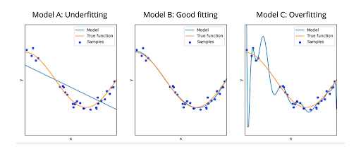
Despite being advantageous, the capability of neural networks to optimize over several hundreds of iterations may eventually become a disadvantage. You can imagine this threshold to be something akin to the difference between understanding and memorizing how to solve a particular set of questions. At first, you might just get the overall idea but still incorrectly answer the majority of questions (underfitting). With more practice, you may reach a point where you are comfortable with the content and can correctly answer most of the questions (good fitting). Here is where you should stop, congratulate yourself, and move onto another fresh set of practice questions. If you keep practicing even further with the same set, however, then you might memorize the answers and end up not getting a grasp of their reasoning at all (overfitting).
In more scientific terms, the accuracy of the neural network greatly decreases when it is overfitting. Although the network still seems to yield good results for the training set, it becomes evidently poor in accuracy when it tries to model new datasets. You can see an example of the three fitting scenarios previously discussed in the diagram below.
Comparing the Neural Network's output for the training and testing set is a popular way to check for overtraining. The code below will plot the Neural Network's output for each class, as well as overlaying it with the output in the training set.
decisions = [] # list to hold decisions of classifier
for X,y in ((X_train, y_train), (X_test, y_test)): # train and test
    d1 = ml_classifier.predict_proba(X[y<0.5])[:, 1] # background
    d2 = ml_classifier.predict_proba(X[y>0.5])[:, 1] # signal
    decisions += [d1, d2] # add to list of classifier decision

highest_decision = max(numpy.max(d) for d in decisions) # get maximum score
bin_edges = [] # list to hold bin edges
bin_edge = -0.1 # start counter for bin_edges
while bin_edge < highest_decision: # up to highest score
    bin_edge += 0.1 # increment
    bin_edges.append(bin_edge)

matplotlib.pyplot.hist(decisions[0], # background in train set
         bins=bin_edges, # lower and upper range of the bins
         density=True, # area under the histogram will sum to 1
         histtype='stepfilled', # lineplot that's filled
         color='red', label='Background (train)', # Background (train)
        alpha=0.5 ) # half transparency
matplotlib.pyplot.hist(decisions[1], # background in train set
         bins=bin_edges, # lower and upper range of the bins
         density=True, # area under the histogram will sum to 1
         histtype='stepfilled', # lineplot that's filled
         color='purple', label='Signal (train)', # Signal (train)
        alpha=0.5 ) # half transparency

hist_background, bin_edges = numpy.histogram(decisions[2], # background test
                                          bins=bin_edges, # number of bins in function definition
                                          density=True ) # area under the histogram will sum to 1

scale = len(decisions[2]) / sum(hist_background) # between raw and normalised
err_background = numpy.sqrt(hist_background * scale) / scale # error on test background

width = 0.1 # histogram bin width
center = (bin_edges[:-1] + bin_edges[1:]) / 2 # bin centres

matplotlib.pyplot.errorbar(x=center, y=hist_background, yerr=err_background, fmt='o', # circles
             c='red', label='Background (test)' ) # Background (test)

hist_signal, bin_edges = numpy.histogram(decisions[3], # siganl test
                                      bins=bin_edges, # number of bins in function definition
                                      density=True ) # area under the histogram will sum to 1
scale = len(decisions[3]) / sum(hist_signal) # between raw and normalised
err_signal = numpy.sqrt(hist_signal * scale) / scale # error on test background

matplotlib.pyplot.errorbar(x=center, y=hist_signal, yerr=err_signal, fmt='*', # circles
             c='purple', label='Signal (test)' ) # Signal (test)

matplotlib.pyplot.xlabel("Neural Network output") # write x-axis label
matplotlib.pyplot.ylabel("Arbitrary units") # write y-axis label
matplotlib.pyplot.legend() # add legend
If overtraining were present, the dots/stars (test set) would be very far from the bars (training set).
Within uncertainties, our dots and stars are in reasonable agreement with our bars, so we can proceed :)
The Universality Theorem
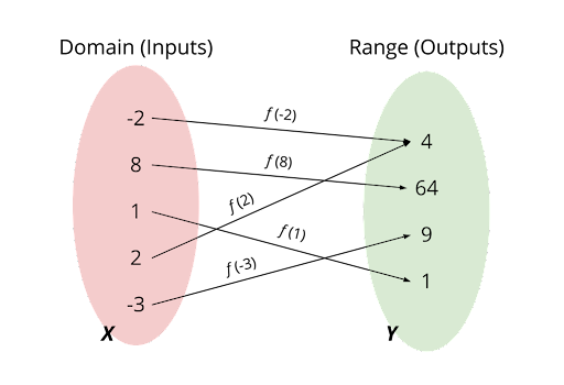
Functions are one of the key principles of Mathematics. You can think of them as a machine that takes some input and processes it into an output. If $f$ is a function, with $X$ its domain (inputs) and $Y$ its range (outputs) such that $f:X \rightarrow Y$. Below you can see a diagram showing links between inputs and outputs allowed by a function. Can you guess the algebraic notation of this function? Because of this general definition, there is a broad scope of actions that can be categorized as functions!
The powerful thing about neural networks is that they can harvest a vast range of real-world applications from functions. The Universality theorem states that “a neural network is theoretically capable of computing an approximation of any function”.
We can observe a similar theorem in human society. A child learns virtually any language that is consistently around them. According to what they experience, each child will acquire a mother tongue. However, no one will ever speak nor write in the same exact way. The very concept of an ideal version of a language is intuitively strange to us. Since we observe several different vocabularies and pronunciations, we render our communication as an unique and approximate expression of a shared language framework.
A neural network works in a similar manner. It will never model a function exactly but it will reach an unique approximation of a function, such as our imaginary network of friends. Be it predicting the existence of planetary bodies from astronomical observations, modelling the structure of a vital protein molecule from chemical data, or probing invisible dark matter from ATLAS Open Data, neural networks can tackle the challenge! That does not mean we will ever find such a model but at least we know they could theoretically do so if given enough computational resources. It is for this reason these algorithms are so ubiquitous in the modern world. More than a pile of mathematics and computations, neural networks are a key tool for human progress in Science.
Going further
If you want to go further, there are a number of things you could try. Try each of these one by one:
- A different Dark Matter signal in "Processes". Change 'DM_300' to one of 'DM_10', 'DM_100', 'DM_200', 'DM_400', 'DM_500', 'DM_600', 'DM_700', 'DM_800', 'DM_2000'.
- Make colourful graphs of the other variables present in your datasets.
- Change variables used by your Neural Network in "Neural Network variables". A "#" at the start of a line means that variable isn't currently being used.
- Modify some Neural Network parameters in "Training the Neural Network model". Use sklearn documentation for some ideas. Perphaps start with parameters such as learning_rate that were discussed in "After All, How do Machines Learn?".
- A different Scaler in "Data Preprocessing". Use sklearn documentation for some ideas.
- A different Machine Learning classifier than
neural_network.MLPClassiferin "Training your Neural Network model". Use sklearn documentation for some ideas. - A different Machine Learning library than
sklearnin "Training your Neural Network model". You could google "machine learning libraries in python".
With each change, keep an eye on significance scores that can be achieved.
Note that we've trained and tested our Neural Network on simulated data. We would then apply it to real experimental data to see if Dark Matter processes are actually seen in real experimental data.