Working with big data: xarray and dask (DEMO)
DS Python for GIS and Geoscience
October, 2020© 2020, Joris Van den Bossche and Stijn Van Hoey. Licensed under CC BY 4.0 Creative Commons
Throughout the course, we worked with small, often simplified or subsampled data. In practice, the tools we have seen still work well with data that fit easily in memory. But also for data larger than memory (e.g. large or high resolution climate data), we can still use many of the familiar tools.
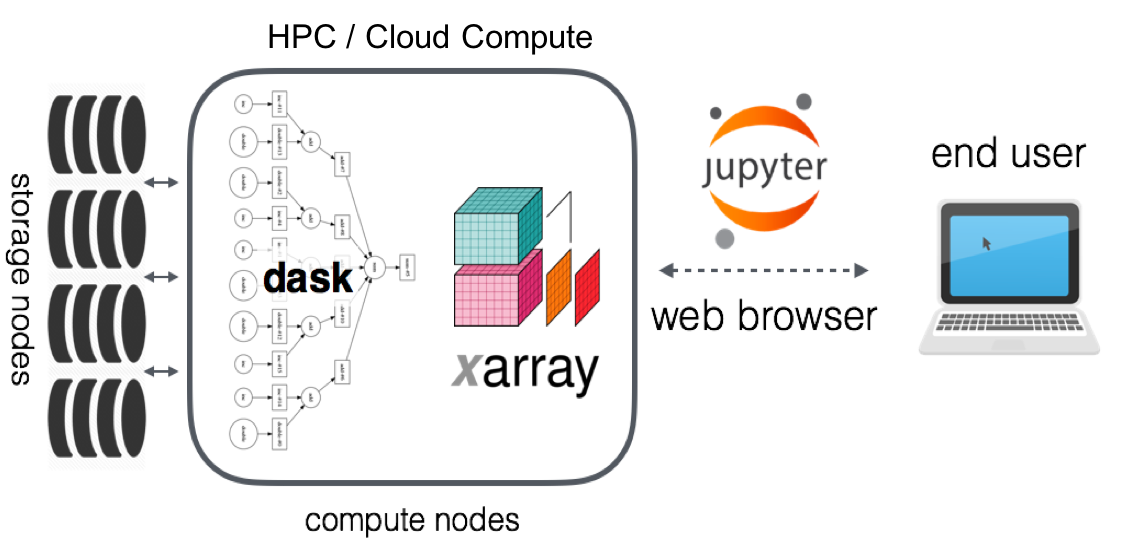
This notebooks includes a brief showcase of using xarray with dask, a package to scale Python workflows (https://dask.org/). Dask integrates very well with xarray, providing a familiar xarray workflow for working with large datasets in parallel or on clusters.
from dask.distributed import Client, LocalCluster
client = Client(LocalCluster(processes=False))  # set up local cluster on your laptop
client
Client
|
Cluster
|
The Multi-Scale Ultra High Resolution (MUR) Sea Surface Temperature (SST) dataset (https://registry.opendata.aws/mur/) provides freely available, global, gap-free, gridded, daily, 1 km data on sea surface temperate for the last 20 years. I downloaded a tiny part this dataset (8 days of 2020) to my local laptop, and stored a subset of the variables (only the "sst" itself) in the zarr format (https://zarr.readthedocs.io/en/stable/), so we can efficiently read it with xarray and dask:
import xarray as xr
ds = xr.open_zarr("data/mur_sst_zarr/")
ds
<xarray.Dataset>
Dimensions:       (lat: 17999, lon: 36000, time: 8)
Coordinates:
  * lat           (lat) float32 -89.99 -89.98 -89.97 ... 89.97 89.98 89.99
  * lon           (lon) float32 -179.99 -179.98 -179.97 ... 179.98 179.99 180.0
  * time          (time) datetime64[ns] 2020-01-01T09:00:00 ... 2020-01-08T09...
Data variables:
    analysed_sst  (time, lat, lon) float32 dask.array<chunksize=(1, 5000, 5000), meta=np.ndarray>
Attributes:
    Conventions:                CF-1.7
    Metadata_Conventions:       Unidata Observation Dataset v1.0
    acknowledgment:             Please acknowledge the use of these data with...
    cdm_data_type:              grid
    comment:                    MUR = "Multi-scale Ultra-high Resolution"
    creator_email:              ghrsst@podaac.jpl.nasa.gov
    creator_name:               JPL MUR SST project
    creator_url:                http://mur.jpl.nasa.gov
    date_created:               20200124T151031Z
    easternmost_longitude:      180.0
    file_quality_level:         3
    gds_version_id:             2.0
    geospatial_lat_resolution:  0.009999999776482582
    geospatial_lat_units:       degrees north
    geospatial_lon_resolution:  0.009999999776482582
    geospatial_lon_units:       degrees east
    history:                    created at nominal 4-day latency; replaced nr...
    id:                         MUR-JPL-L4-GLOB-v04.1
    institution:                Jet Propulsion Laboratory
    keywords:                   Oceans > Ocean Temperature > Sea Surface Temp...
    keywords_vocabulary:        NASA Global Change Master Directory (GCMD) Sc...
    license:                    These data are available free of charge under...
    metadata_link:              http://podaac.jpl.nasa.gov/ws/metadata/datase...
    naming_authority:           org.ghrsst
    netcdf_version_id:          4.1
    northernmost_latitude:      90.0
    platform:                   Terra, Aqua, GCOM-W, MetOp-A, MetOp-B, Buoys/...
    processing_level:           L4
    product_version:            04.1
    project:                    NASA Making Earth Science Data Records for Us...
    publisher_email:            ghrsst-po@nceo.ac.uk
    publisher_name:             GHRSST Project Office
    publisher_url:              http://www.ghrsst.org
    references:                 http://podaac.jpl.nasa.gov/Multi-scale_Ultra-...
    sensor:                     MODIS, AMSR2, AVHRR, in-situ
    source:                     MODIS_T-JPL, MODIS_A-JPL, AMSR2-REMSS, AVHRRM...
    southernmost_latitude:      -90.0
    spatial_resolution:         0.01 degrees
    standard_name_vocabulary:   NetCDF Climate and Forecast (CF) Metadata Con...
    start_time:                 20200108T090000Z
    stop_time:                  20200108T090000Z
    summary:                    A merged, multi-sensor L4 Foundation SST anal...
    time_coverage_end:          20200108T210000Z
    time_coverage_start:        20200107T210000Z
    title:                      Daily MUR SST, Final product
    uuid:                       27665bc0-d5fc-11e1-9b23-0800200c9a66
westernmost_longitude: -180.0- lat: 17999
- lon: 36000
- time: 8
- lat(lat)float32-89.99 -89.98 ... 89.98 89.99
- axis :
- Y
- comment :
- geolocations inherited from the input data without correction
- long_name :
- latitude
- standard_name :
- latitude
- units :
- degrees_north
- valid_max :
- 90.0
- valid_min :
- -90.0
array([-89.99, -89.98, -89.97, ..., 89.97, 89.98, 89.99], dtype=float32)
- lon(lon)float32-179.99 -179.98 ... 179.99 180.0
- axis :
- X
- comment :
- geolocations inherited from the input data without correction
- long_name :
- longitude
- standard_name :
- longitude
- units :
- degrees_east
- valid_max :
- 180.0
- valid_min :
- -180.0
array([-179.99, -179.98, -179.97, ..., 179.98, 179.99, 180. ], dtype=float32) - time(time)datetime64[ns]2020-01-01T09:00:00 ... 2020-01-...
- axis :
- T
- comment :
- Nominal time of analyzed fields
- long_name :
- reference time of sst field
- standard_name :
- time
array(['2020-01-01T09:00:00.000000000', '2020-01-02T09:00:00.000000000',
       '2020-01-03T09:00:00.000000000', '2020-01-04T09:00:00.000000000',
       '2020-01-05T09:00:00.000000000', '2020-01-06T09:00:00.000000000',
       '2020-01-07T09:00:00.000000000', '2020-01-08T09:00:00.000000000'],
      dtype='datetime64[ns]')
- analysed_sst(time, lat, lon)float32dask.array<chunksize=(1, 5000, 5000), meta=np.ndarray>
- comment :
- "Final" version using Multi-Resolution Variational Analysis (MRVA) method for interpolation
- long_name :
- analysed sea surface temperature
- source :
- MODIS_T-JPL, MODIS_A-JPL, AMSR2-REMSS, AVHRRMTA_G-NAVO, AVHRRMTB_G-NAVO, iQUAM-NOAA/NESDIS, Ice_Conc-OSISAF
- standard_name :
- sea_surface_foundation_temperature
- units :
- kelvin
- valid_max :
- 32767
- valid_min :
- -32767
Array Chunk Bytes 20.73 GB 100.00 MB Shape (8, 17999, 36000) (1, 5000, 5000) Count 257 Tasks 256 Chunks Type float32 numpy.ndarray
- Conventions :
- CF-1.7
- Metadata_Conventions :
- Unidata Observation Dataset v1.0
- acknowledgment :
- Please acknowledge the use of these data with the following statement: These data were provided by JPL under support by NASA MEaSUREs program.
- cdm_data_type :
- grid
- comment :
- MUR = "Multi-scale Ultra-high Resolution"
- creator_email :
- ghrsst@podaac.jpl.nasa.gov
- creator_name :
- JPL MUR SST project
- creator_url :
- http://mur.jpl.nasa.gov
- date_created :
- 20200124T151031Z
- easternmost_longitude :
- 180.0
- file_quality_level :
- 3
- gds_version_id :
- 2.0
- geospatial_lat_resolution :
- 0.009999999776482582
- geospatial_lat_units :
- degrees north
- geospatial_lon_resolution :
- 0.009999999776482582
- geospatial_lon_units :
- degrees east
- history :
- created at nominal 4-day latency; replaced nrt (1-day latency) version.
- id :
- MUR-JPL-L4-GLOB-v04.1
- institution :
- Jet Propulsion Laboratory
- keywords :
- Oceans > Ocean Temperature > Sea Surface Temperature
- keywords_vocabulary :
- NASA Global Change Master Directory (GCMD) Science Keywords
- license :
- These data are available free of charge under data policy of JPL PO.DAAC.
- metadata_link :
- http://podaac.jpl.nasa.gov/ws/metadata/dataset/?format=iso&shortName=MUR-JPL-L4-GLOB-v04.1
- naming_authority :
- org.ghrsst
- netcdf_version_id :
- 4.1
- northernmost_latitude :
- 90.0
- platform :
- Terra, Aqua, GCOM-W, MetOp-A, MetOp-B, Buoys/Ships
- processing_level :
- L4
- product_version :
- 04.1
- project :
- NASA Making Earth Science Data Records for Use in Research Environments (MEaSUREs) Program
- publisher_email :
- ghrsst-po@nceo.ac.uk
- publisher_name :
- GHRSST Project Office
- publisher_url :
- http://www.ghrsst.org
- references :
- http://podaac.jpl.nasa.gov/Multi-scale_Ultra-high_Resolution_MUR-SST
- sensor :
- MODIS, AMSR2, AVHRR, in-situ
- source :
- MODIS_T-JPL, MODIS_A-JPL, AMSR2-REMSS, AVHRRMTA_G-NAVO, AVHRRMTB_G-NAVO, iQUAM-NOAA/NESDIS, Ice_Conc-OSISAF
- southernmost_latitude :
- -90.0
- spatial_resolution :
- 0.01 degrees
- standard_name_vocabulary :
- NetCDF Climate and Forecast (CF) Metadata Convention
- start_time :
- 20200108T090000Z
- stop_time :
- 20200108T090000Z
- summary :
- A merged, multi-sensor L4 Foundation SST analysis product from JPL.
- time_coverage_end :
- 20200108T210000Z
- time_coverage_start :
- 20200107T210000Z
- title :
- Daily MUR SST, Final product
- uuid :
- 27665bc0-d5fc-11e1-9b23-0800200c9a66
- westernmost_longitude :
- -180.0
Looking at the actual sea surface temperature DataArray:
ds.analysed_sst
<xarray.DataArray 'analysed_sst' (time: 8, lat: 17999, lon: 36000)>
dask.array<zarr, shape=(8, 17999, 36000), dtype=float32, chunksize=(1, 5000, 5000), chunktype=numpy.ndarray>
Coordinates:
  * lat      (lat) float32 -89.99 -89.98 -89.97 -89.96 ... 89.97 89.98 89.99
  * lon      (lon) float32 -179.99 -179.98 -179.97 ... 179.98 179.99 180.0
  * time     (time) datetime64[ns] 2020-01-01T09:00:00 ... 2020-01-08T09:00:00
Attributes:
    comment:        "Final" version using Multi-Resolution Variational Analys...
    long_name:      analysed sea surface temperature
    source:         MODIS_T-JPL, MODIS_A-JPL, AMSR2-REMSS, AVHRRMTA_G-NAVO, A...
    standard_name:  sea_surface_foundation_temperature
    units:          kelvin
    valid_max:      32767
valid_min: -32767- time: 8
- lat: 17999
- lon: 36000
- dask.array<chunksize=(1, 5000, 5000), meta=np.ndarray>
Array Chunk Bytes 20.73 GB 100.00 MB Shape (8, 17999, 36000) (1, 5000, 5000) Count 257 Tasks 256 Chunks Type float32 numpy.ndarray - lat(lat)float32-89.99 -89.98 ... 89.98 89.99
- axis :
- Y
- comment :
- geolocations inherited from the input data without correction
- long_name :
- latitude
- standard_name :
- latitude
- units :
- degrees_north
- valid_max :
- 90.0
- valid_min :
- -90.0
array([-89.99, -89.98, -89.97, ..., 89.97, 89.98, 89.99], dtype=float32)
- lon(lon)float32-179.99 -179.98 ... 179.99 180.0
- axis :
- X
- comment :
- geolocations inherited from the input data without correction
- long_name :
- longitude
- standard_name :
- longitude
- units :
- degrees_east
- valid_max :
- 180.0
- valid_min :
- -180.0
array([-179.99, -179.98, -179.97, ..., 179.98, 179.99, 180. ], dtype=float32) - time(time)datetime64[ns]2020-01-01T09:00:00 ... 2020-01-...
- axis :
- T
- comment :
- Nominal time of analyzed fields
- long_name :
- reference time of sst field
- standard_name :
- time
array(['2020-01-01T09:00:00.000000000', '2020-01-02T09:00:00.000000000',
       '2020-01-03T09:00:00.000000000', '2020-01-04T09:00:00.000000000',
       '2020-01-05T09:00:00.000000000', '2020-01-06T09:00:00.000000000',
       '2020-01-07T09:00:00.000000000', '2020-01-08T09:00:00.000000000'],
      dtype='datetime64[ns]')
- comment :
- "Final" version using Multi-Resolution Variational Analysis (MRVA) method for interpolation
- long_name :
- analysed sea surface temperature
- source :
- MODIS_T-JPL, MODIS_A-JPL, AMSR2-REMSS, AVHRRMTA_G-NAVO, AVHRRMTB_G-NAVO, iQUAM-NOAA/NESDIS, Ice_Conc-OSISAF
- standard_name :
- sea_surface_foundation_temperature
- units :
- kelvin
- valid_max :
- 32767
- valid_min :
- -32767
The representation already indicated that this DataArray (although being a tiny part of the actual full dataset) is quite big: 20.7 GB if loaded fully into memory at once (which would not fit in the memory of my laptop).
The xarray.DataArray is now backed by a dask array instead of a numpy array. This allows us to do computations on the large data in chunked way.
For example, let's compute the overall average temperature for the full globe for each timestep:
overall_mean = ds.analysed_sst.mean(dim=("lon", "lat"))
overall_mean
<xarray.DataArray 'analysed_sst' (time: 8)>
dask.array<mean_agg-aggregate, shape=(8,), dtype=float32, chunksize=(1,), chunktype=numpy.ndarray>
Coordinates:
  * time     (time) datetime64[ns] 2020-01-01T09:00:00 ... 2020-01-08T09:00:00
- time: 8
- dask.array<chunksize=(1,), meta=np.ndarray>
Array Chunk Bytes 32 B 4 B Shape (8,) (1,) Count 601 Tasks 8 Chunks Type float32 numpy.ndarray - time(time)datetime64[ns]2020-01-01T09:00:00 ... 2020-01-...
- axis :
- T
- comment :
- Nominal time of analyzed fields
- long_name :
- reference time of sst field
- standard_name :
- time
array(['2020-01-01T09:00:00.000000000', '2020-01-02T09:00:00.000000000',
       '2020-01-03T09:00:00.000000000', '2020-01-04T09:00:00.000000000',
       '2020-01-05T09:00:00.000000000', '2020-01-06T09:00:00.000000000',
       '2020-01-07T09:00:00.000000000', '2020-01-08T09:00:00.000000000'],
      dtype='datetime64[ns]')
This returned a lazy object, and not yet computed the actual average. Let's explicitly compute it:
%%time
overall_mean.compute()
CPU times: user 1min 56s, sys: 46.3 s, total: 2min 42s
Wall time: 31.5 s
<xarray.DataArray 'analysed_sst' (time: 8)>
array([287.08176, 287.08545, 287.0962 , 287.09042, 287.08246, 287.07053,
       287.08984, 287.1125 ], dtype=float32)
Coordinates:
* time (time) datetime64[ns] 2020-01-01T09:00:00 ... 2020-01-08T09:00:00- time: 8
- 287.08176 287.08545 287.0962 ... 287.07053 287.08984 287.1125
array([287.08176, 287.08545, 287.0962 , 287.09042, 287.08246, 287.07053, 287.08984, 287.1125 ], dtype=float32) - time(time)datetime64[ns]2020-01-01T09:00:00 ... 2020-01-...
- axis :
- T
- comment :
- Nominal time of analyzed fields
- long_name :
- reference time of sst field
- standard_name :
- time
array(['2020-01-01T09:00:00.000000000', '2020-01-02T09:00:00.000000000',
       '2020-01-03T09:00:00.000000000', '2020-01-04T09:00:00.000000000',
       '2020-01-05T09:00:00.000000000', '2020-01-06T09:00:00.000000000',
       '2020-01-07T09:00:00.000000000', '2020-01-08T09:00:00.000000000'],
      dtype='datetime64[ns]')
This takes some time, but it did run on my laptop even while the dataset did not fit in the memory of my laptop.
Integrating with hvplot and datashader, we can also still interactively plot and explore the large dataset:
import hvplot.xarray
ds.analysed_sst.isel(time=-1).hvplot.quadmesh(
    'lon', 'lat', rasterize=True, dynamic=True,
    width=800, height=450, cmap='RdBu_r')
Zooming in on this figure we re-read and rasterize the subset we are viewing to provide a higher resolution image.
As a summary, using dask with xarray allows:
- to use the familiar xarray workflows for larger data as well
- use the same code to work on our laptop or on a big cluster
PANGEO: A community platform for Big Data geoscience
Website: https://pangeo.io/index.html
They have a gallery with many interesting examples, many of them using this combination of xarray and dask.
Pangeo focuses primarily on cloud computing (storing the big datasets in cloud-native file formats and also doing the computations in the cloud), but all the tools like xarray and dask developed by this community and shown in the examples also work on your laptop or university's cluster.