AI4M Course 1 week 3 lecture notebook
U-Net model
In this week's assignment, you'll be using a network architecture called "U-Net". The name of this network architecture comes from it's U-like shape when shown in a diagram like this (image from U-net entry on wikipedia):
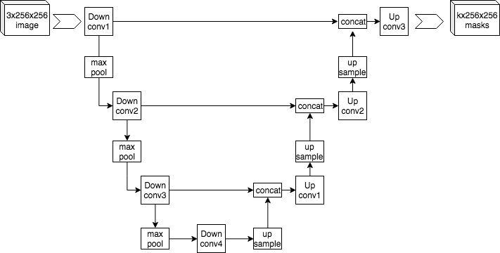
U-nets are commonly used for image segmentation, which will be your task in the upcoming assignment. You won't actually need to implement U-Net in the assignment, but we wanted to give you an opportunity to gain some familiarity with this architecture here before you use it in the assignment.
As you can see from the diagram, this architecture features a series of down-convolutions connected by max-pooling operations, followed by a series of up-convolutions connected by upsampling and concatenation operations. Each of the down-convolutions is also connected directly to the concatenation operations in the upsampling portion of the network. For more detail on the U-Net architecture, have a look at the original U-Net paper by Ronneberger et al. 2015.
In this lab, you'll create a basic U-Net using Keras.
# Import the elements you'll need to build your U-Net
import keras
from keras import backend as K
from keras.engine import Input, Model
from keras.layers import Conv3D, MaxPooling3D, UpSampling3D, Activation, BatchNormalization, PReLU, Deconvolution3D
from keras.optimizers import Adam
from keras.layers.merge import concatenate
# Set the image shape to have the channels in the first dimension
K.set_image_data_format("channels_first")
Using TensorFlow backend.
The "depth" of your U-Net
The "depth" of your U-Net is equal to the number of down-convolutions you will use. In the image above, the depth is 4 because there are 4 down-convolutions running down the left side including the very bottom of the U.
For this exercise, you'll use a U-Net depth of 2, meaning you'll have 2 down-convolutions in your network.
Input layer and its "depth"
In this lab and in the assignment, you will be doing 3D image segmentation, which is to say that, in addition to "height" and "width", your input layer will also have a "length". We are deliberately using the word "length" instead of "depth" here to describe the third spatial dimension of the input so as not to confuse it with the depth of the network as defined above.
The shape of the input layer is (num_channels, height, width, length), where num_channels you can think of like color channels in an image, height, width and length are just the size of the input.
For the assignment, the values will be:
- num_channels: 4
- height: 160
- width: 160
- length: 16
# Define an input layer tensor of the shape you'll use in the assignment
input_layer = Input(shape=(4, 160, 160, 16))
input_layer
<tf.Tensor 'input_1:0' shape=(?, 4, 160, 160, 16) dtype=float32>
Notice that the tensor shape has a '?' as the very first dimension. This will be the batch size. So the dimensions of the tensor are: (batch_size, num_channels, height, width, length)
Contracting (downward) path
Here you'll start by constructing the downward path in your network (the left side of the U-Net). The (height, width, length) of the input gets smaller as you move down this path, and the number of channels increases.
Depth 0
By "depth 0" here, we're referring to the depth of the first down-convolution in the U-net.
The number of filters is specified for each depth and for each layer within that depth.
The formula to use for calculating the number of filters is: $$filters_{i} = 32 \times (2^{i})$$
Where $i$ is the current depth.
So at depth $i=0$: $$filters_{0} = 32 \times (2^{0}) = 32$$
Layer 0
There are two convolutional layers for each depth
Run the next cell to create the first 3D convolution
# Define a Conv3D tensor with 32 filters
down_depth_0_layer_0 = Conv3D(filters=32,
                              kernel_size=(3,3,3),
                              padding='same',
                              strides=(1,1,1)
                              )(input_layer)
down_depth_0_layer_0
Notice that with 32 filters, the result you get above is a tensor with 32 channels.
Run the next cell to add a relu activation to the first convolutional layer
# Add a relu activation to layer 0 of depth 0
down_depth_0_layer_0 = Activation('relu')(down_depth_0_layer_0)
down_depth_0_layer_0
Depth 0, Layer 1
For layer 1 of depth 0, the formula for calculating the number of filters is: $$filters_{i} = 32 \times (2^{i}) \times 2$$
Where $i$ is the current depth.
- Notice that the '$\times~2$' at the end of this expression isn't there for layer 0.
So at depth $i=0$ for layer 1: $$filters_{0} = 32 \times (2^{0}) \times 2 = 64$$
# Create a Conv3D layer with 64 filters and add relu activation
down_depth_0_layer_1 = Conv3D(filters=64,
                kernel_size=(3,3,3),
                padding='same',
                strides=(1,1,1)
               )(down_depth_0_layer_0)
down_depth_0_layer_1 = Activation('relu')(down_depth_0_layer_1)
down_depth_0_layer_1
Max pooling
Within the U-Net architecture, there is a max pooling operation after each of the down-convolutions (not including the last down-convolution at the bottom of the U). In general, this means you'll add max pooling after each down-convolution up to (but not including) the depth - 1 down-convolution (since you started counting at 0).
For this lab exercise:
- The overall depth of the U-Net you're constructing is 2
- So the bottom of your U is at a depth index of: $2-1 = 1$.
- So far you've only defined the $depth=0$ down-convolutions, so the next thing to do is add max pooling
Run the next cell to add a max pooling operation to your U-Net
# Define a max pooling layer
down_depth_0_layer_pool = MaxPooling3D(pool_size=(2,2,2))(down_depth_0_layer_1)
down_depth_0_layer_pool
Depth 1, Layer 0
At depth 1, layer 0, the formula for calculating the number of filters is: $$filters_{i} = 32 \times (2^{i})$$
Where $i$ is the current depth.
So at depth $i=1$: $$filters_{1} = 32 \times (2^{1}) = 64$$
Run the next cell to add a Conv3D layer to your network with relu activation
# Add a Conv3D layer to your network with relu activation
down_depth_1_layer_0 = Conv3D(filters=64,
                kernel_size=(3,3,3),
                padding='same',
                strides=(1,1,1)
               )(down_depth_0_layer_pool)
down_depth_1_layer_0 = Activation('relu')(down_depth_1_layer_0)
down_depth_1_layer_0
Depth 1, Layer 1
For layer 1 of depth 1 the formula you'll use for number of filters is: $$filters_{i} = 32 \times (2^{i}) \times 2$$
Where $i$ is the current depth.
- Notice that the '$\times 2$' at the end of this expression isn't there for layer 0.
So at depth $i=1$: $$filters_{0} = 32 \times (2^{1}) \times 2 = 128$$
Run the next cell to add another Conv3D with 128 filters to your network.
# Add another Conv3D with 128 filters to your network.
down_depth_1_layer_1 = Conv3D(filters=128,
                kernel_size=(3,3,3),
                padding='same',
                strides=(1,1,1)
               )(down_depth_1_layer_0)
down_depth_1_layer_1 = Activation('relu')(down_depth_1_layer_1)
down_depth_1_layer_1
No max pooling at depth 1 (the bottom of the U)
When you get to the "bottom" of the U-net, you don't need to apply max pooling after the convolutions.
Expanding (upward) Path
Now you'll work on the expanding path of the U-Net, (going up on the right side, when viewing the diagram). The image's (height, width, length) all get larger in the expanding path.
Depth 0, Up sampling layer 0
You'll use a pool size of (2,2,2) for upsampling.
- This is the default value for tf.keras.layers.UpSampling3D
- As input to the upsampling at depth 1, you'll use the last layer of the downsampling. In this case, it's the depth 1 layer 1.
Run the next cell to add an upsampling operation to your network. Note that you're not adding any activation to this upsampling layer.
# Add an upsampling operation to your network
up_depth_0_layer_0 = UpSampling3D(size=(2,2,2))(down_depth_1_layer_1)
up_depth_0_layer_0
Concatenate upsampled depth 0 with downsampled depth 0
Now you'll apply a concatenation operation using the layers that are both at the same depth of 0.
up_depth_0_layer_0: shape is (?, 128, 160, 160, 16)
depth_0_layer_1: shape is (?, 64, 160, 160, 16)
Double check that both of these layers have the same height, width and length.
If they're the same, then they can be concatenated along axis 1 (the channel axis).
The (height, width, length) is (160, 160, 16) for both.
Run the next cell to check that the layers you wish to concatenate have the same height, width and length.
# Print the shape of layers to concatenate
print(up_depth_0_layer_0)
print()
print(down_depth_0_layer_1)
Run the next cell to add a concatenation operation to your network
# Add a concatenation along axis 1
up_depth_1_concat = concatenate([up_depth_0_layer_0,
                                 down_depth_0_layer_1],
                                axis=1)
up_depth_1_concat
Notice that the upsampling layer had 128 channels, and the down-convolution layer had 64 channels so that when concatenated, the result has 128 + 64 = 192 channels.
Up-convolution layer 1
The number of filters for this layer will be set to the number of channels in the down-convolution's layer 1 at the same depth of 0 (down_depth_0_layer_1).
Run the next cell to have a look at the shape of the down-convolution depth 0 layer 1
down_depth_0_layer_1
Notice the number of channels for depth_0_layer_1 is 64
print(f"number of filters: {down_depth_0_layer_1._keras_shape[1]}")
# Add a Conv3D up-convolution with 64 filters to your network
up_depth_1_layer_1 = Conv3D(filters=64,
                            kernel_size=(3,3,3),
                            padding='same',
                            strides=(1,1,1)
                           )(up_depth_1_concat)
up_depth_1_layer_1 = Activation('relu')(up_depth_1_layer_1)
up_depth_1_layer_1
Up-convolution depth 0, layer 2
At layer 2 of depth 0 in the up-convolution the next step will be to add another up-convolution. The number of filters you'll want to use for this next up-convolution will need to be equal to the number of filters in the down-convolution depth 0 layer 1.
Run the next cell to remind yourself of the number of filters in down-convolution depth 0 layer 1.
print(down_depth_0_layer_1)
print(f"number of filters: {down_depth_0_layer_1._keras_shape[1]}")
As you can see, the number of channels / filters in down_depth_0_layer_1 is 64.
Run the next cell to add a Conv3D up-convolution with 64 filters to your network.
# Add a Conv3D up-convolution with 64 filters to your network
up_depth_1_layer_2 = Conv3D(filters=64,
                            kernel_size=(3,3,3),
                            padding='same',
                            strides=(1,1,1)
                           )(up_depth_1_layer_1)
up_depth_1_layer_2 = Activation('relu')(up_depth_1_layer_2)
up_depth_1_layer_2
Final Convolution
For the final convolution, you will set the number of filters to be equal to the number of classes in your input data.
In the assignment, you will be using data with 3 classes, namely:
- 1: edema
- 2: non-enhancing tumor
- 3: enhancing tumor
Run the next cell to add a final Conv3D with 3 filters to your network.
# Add a final Conv3D with 3 filters to your network.
final_conv = Conv3D(filters=3, #3 categories
                    kernel_size=(1,1,1),
                    padding='valid',
                    strides=(1,1,1)
                    )(up_depth_1_layer_2)
final_conv
Activation for final convolution
Run the next cell to add a sigmoid activation to your final convolution.
# Add a sigmoid activation to your final convolution.
final_activation = Activation('sigmoid')(final_conv)
final_activation
Create and compile the model
In this example, you will be setting the loss and metrics to options that are pre-built in Keras. However, in the assignment, you will implement better loss functions and metrics for evaluating the model's performance.
Run the next cell to define and compile your model based on the architecture you created above.
# Define and compile your model
model = Model(inputs=input_layer, outputs=final_activation)
model.compile(optimizer=Adam(lr=0.00001),
              loss='categorical_crossentropy',
              metrics=['categorical_accuracy']
             )
# Print out a summary of the model you created
model.summary()
Congratulations! You've created your very own U-Net model architecture!
Next, you'll check that you did everything correctly by comparing your model summary to the example model defined below.
Double check your model
To double check that you created the correct model, use a function that we've provided to create the same model, and check that the layers and the layer dimensions match!
# Import predefined utilities
import util
# Create a model using a predefined function
model_2 = util.unet_model_3d(depth=2,
                                loss_function='categorical_crossentropy',
                                metrics=['categorical_accuracy'])
# Print out a summary of the model created by the predefined function
model_2.summary()
Look at the model summary for the U-Net you created and compare it to the summary for the example model created by the predefined function you imported above.
That's it for this exercise, we hope this have provided you with more insight into the network architecture you'll be working with in this week's assignment!