20 - Deep Learning using keras
by Alejandro Correa Bahnsen and Jesus Solano
version 1.4, May 2019
Part of the class Practical Machine Learning
This notebook is licensed under a Creative Commons Attribution-ShareAlike 3.0 Unported License. Special thanks goes to Valerio Maggio, Fondazione Bruno Kessler
Keras: Deep Learning library for Theano and TensorFlow
Keras is a minimalist, highly modular neural networks library, written in Python and capable of running on top of either TensorFlow or Theano.
It was developed with a focus on enabling fast experimentation. Being able to go from idea to result with the least possible delay is key to doing good research.
ref: https://keras.io/
Boston Housing Data
from sklearn.datasets import load_boston
boston_dataset = load_boston()
print(boston_dataset.DESCR)
.. _boston_dataset:

Boston house prices dataset
---------------------------

**Data Set Characteristics:**

    :Number of Instances: 506

    :Number of Attributes: 13 numeric/categorical predictive. Median Value (attribute 14) is usually the target.

    :Attribute Information (in order):
        - CRIM     per capita crime rate by town
        - ZN       proportion of residential land zoned for lots over 25,000 sq.ft.
        - INDUS    proportion of non-retail business acres per town
        - CHAS     Charles River dummy variable (= 1 if tract bounds river; 0 otherwise)
        - NOX      nitric oxides concentration (parts per 10 million)
        - RM       average number of rooms per dwelling
        - AGE      proportion of owner-occupied units built prior to 1940
        - DIS      weighted distances to five Boston employment centres
        - RAD      index of accessibility to radial highways
        - TAX      full-value property-tax rate per $10,000
        - PTRATIO  pupil-teacher ratio by town
        - B        1000(Bk - 0.63)^2 where Bk is the proportion of blacks by town
        - LSTAT    % lower status of the population
        - MEDV     Median value of owner-occupied homes in $1000's

    :Missing Attribute Values: None

    :Creator: Harrison, D. and Rubinfeld, D.L.

This is a copy of UCI ML housing dataset.
https://archive.ics.uci.edu/ml/machine-learning-databases/housing/


This dataset was taken from the StatLib library which is maintained at Carnegie Mellon University.

The Boston house-price data of Harrison, D. and Rubinfeld, D.L. 'Hedonic
prices and the demand for clean air', J. Environ. Economics & Management,
vol.5, 81-102, 1978.   Used in Belsley, Kuh & Welsch, 'Regression diagnostics
...', Wiley, 1980.   N.B. Various transformations are used in the table on
pages 244-261 of the latter.

The Boston house-price data has been used in many machine learning papers that address regression
problems.

.. topic:: References

   - Belsley, Kuh & Welsch, 'Regression diagnostics: Identifying Influential Data and Sources of Collinearity', Wiley, 1980. 244-261.
   - Quinlan,R. (1993). Combining Instance-Based and Model-Based Learning. In Proceedings on the Tenth International Conference of Machine Learning, 236-243, University of Massachusetts, Amherst. Morgan Kaufmann.
For this section we will use the Boston Housing Data.
Single Layer Neural Network
Data Preparation
import pandas as pd
from sklearn.datasets import load_boston
import numpy as np
import matplotlib.pyplot as plt
from sklearn.model_selection import train_test_split
boston_dataset = load_boston()
boston = pd.DataFrame(boston_dataset.data, columns=boston_dataset.feature_names)

X = boston.drop(boston.columns[-1],axis=1)

Y = pd.DataFrame(np.array(boston_dataset.target), columns=['labels'])

boston.head()
| CRIM | ZN | INDUS | CHAS | NOX | RM | AGE | DIS | RAD | TAX | PTRATIO | B | LSTAT | |
|---|---|---|---|---|---|---|---|---|---|---|---|---|---|
| 0 | 0.00632 | 18.0 | 2.31 | 0.0 | 0.538 | 6.575 | 65.2 | 4.0900 | 1.0 | 296.0 | 15.3 | 396.90 | 4.98 |
| 1 | 0.02731 | 0.0 | 7.07 | 0.0 | 0.469 | 6.421 | 78.9 | 4.9671 | 2.0 | 242.0 | 17.8 | 396.90 | 9.14 |
| 2 | 0.02729 | 0.0 | 7.07 | 0.0 | 0.469 | 7.185 | 61.1 | 4.9671 | 2.0 | 242.0 | 17.8 | 392.83 | 4.03 |
| 3 | 0.03237 | 0.0 | 2.18 | 0.0 | 0.458 | 6.998 | 45.8 | 6.0622 | 3.0 | 222.0 | 18.7 | 394.63 | 2.94 |
| 4 | 0.06905 | 0.0 | 2.18 | 0.0 | 0.458 | 7.147 | 54.2 | 6.0622 | 3.0 | 222.0 | 18.7 | 396.90 | 5.33 |
# Split datasets.
X_train, X_test , Y_train, Y_test = train_test_split(X,Y, test_size=0.3 ,random_state=22)

# Normalize Data
from sklearn.preprocessing import StandardScaler

# Define the Preprocessing Method and Fit Training Data to it
scaler = StandardScaler()
scaler.fit(X)

# Make X_train to be the Scaled Version of Data
# This process scales all the values in all 6 columns and replaces them with the new values
X_train = pd.DataFrame(data=scaler.transform(X_train), columns=X_train.columns, index=X_train.index)
X_test = pd.DataFrame(data=scaler.transform(X_test), columns=X_test.columns, index=X_test.index)

X_train = np.array(X_train)
Y_train = np.array(Y_train)

X_test = np.array(X_test)
Y_test = np.array(Y_test)
# As it is a regression problem the output is a neuron.
output_var = Y_train.shape[1]
print(output_var, ' output variables')

dims = X_train.shape[1]
print(dims, 'input variables')
1  output variables
12 input variables
Y_train.shape
(354, 1)
Using Tensorflow
import tensorflow as tf
# Parameters
learning_rate = 0.01
training_epochs = 150
display_step = 1
# tf Graph Input
x = tf.placeholder(tf.float32, [None, dims])
y = tf.placeholder(tf.float32, [None,1])
# Try to print a placeholder.
x
<tf.Tensor 'Placeholder:0' shape=(?, 12) dtype=float32>
Model (Introducing Tensorboard)
# Construct (linear) model
with tf.name_scope("model") as scope:
    # Set model weights
    W = tf.Variable(tf.zeros([dims, output_var]))
    b = tf.Variable(tf.zeros([output_var]))
    activation = tf.add(tf.matmul(x, W), b) # Softmax

    # Add summary ops to collect data
    w_h = tf.summary.histogram("weights_histogram", W)
    b_h = tf.summary.histogram("biases_histograms", b)
    tf.summary.scalar('mean_weights', tf.reduce_mean(W))
    tf.summary.scalar('mean_bias', tf.reduce_mean(b))

# Minimize error using cross entropy
# Note: More name scopes will clean up graph representation
with tf.name_scope("cost_function") as scope:
    cost = tf.reduce_mean(tf.square(activation-y))
    # Create a summary to monitor the cost function
    tf.summary.scalar("cost_function", cost)
    tf.summary.histogram("cost_histogram", cost)

with tf.name_scope("train") as scope:
    # Set the Optimizer
    optimizer = tf.train.GradientDescentOptimizer(learning_rate).minimize(cost)
Learning in a TF Session
# Launch the graph
with tf.Session() as session:
    # Initializing the variables
    session.run(tf.global_variables_initializer())

    cost_epochs = []
    # Training cycle
    for epoch in range(training_epochs):
        _, c = session.run(fetches=[optimizer, cost], feed_dict={x: X_train, y: Y_train})
        cost_epochs.append(c)
        #writer.add_summary(summary=summary, global_step=epoch)
        #print("accuracy epoch {}:{}".format(epoch, accuracy.eval({x: X_train, y: Y_train})))

        # Print the Loss/Error after every 100 epochs
        if epoch%10 == 0:
            print('Epoch: {0}, Error: {1}'.format(epoch, c))

    print("Training phase finished")

    #plotting
    plt.figure(figsize=(12,8))
    plt.plot(range(len(cost_epochs)), cost_epochs, 'o', label='Logistic Regression Training phase')
    plt.ylabel('cost')
    plt.xlabel('epoch')
    plt.legend()
    plt.show()

    #prediction = tf.argmax(activation, 1)
    #print(prediction.eval({x: X_test}))
Epoch: 0, Error: 579.5443115234375
Epoch: 10, Error: 384.7831115722656
Epoch: 20, Error: 267.9833984375
Epoch: 30, Error: 190.64822387695312
Epoch: 40, Error: 138.649169921875
Epoch: 50, Error: 103.560546875
Epoch: 60, Error: 79.83016967773438
Epoch: 70, Error: 63.743778228759766
Epoch: 80, Error: 52.8095703125
Epoch: 90, Error: 45.35356140136719
Epoch: 100, Error: 40.249916076660156
Epoch: 110, Error: 36.74049758911133
Epoch: 120, Error: 34.31406021118164
Epoch: 130, Error: 32.62529373168945
Epoch: 140, Error: 31.440656661987305
Training phase finished

Using Keras
from keras.models import Sequential
from keras.layers import Dense, Activation
from livelossplot import PlotLossesKeras
from keras import backend as K
Using TensorFlow backend.
K.clear_session()
print("Building model...")

print('Model variables: ', dims)

model = Sequential()
model.add(Dense(output_var, input_shape=(dims,)))

print(model.summary())

model.compile(optimizer='sgd', loss='mean_squared_error')
model.fit(X_train, Y_train, verbose=2,epochs=15)
Building model...
Model variables:  12
_________________________________________________________________
Layer (type)                 Output Shape              Param #
=================================================================
dense_1 (Dense)              (None, 1)                 13
=================================================================
Total params: 13
Trainable params: 13
Non-trainable params: 0
_________________________________________________________________
None
Epoch 1/15
 - 0s - loss: 474.8418
Epoch 2/15
 - 0s - loss: 303.8997
Epoch 3/15
 - 0s - loss: 203.2895
Epoch 4/15
 - 0s - loss: 139.5915
Epoch 5/15
 - 0s - loss: 99.2025
Epoch 6/15
 - 0s - loss: 75.1656
Epoch 7/15
 - 0s - loss: 57.9853
Epoch 8/15
 - 0s - loss: 46.0630
Epoch 9/15
 - 0s - loss: 40.6584
Epoch 10/15
 - 0s - loss: 36.7637
Epoch 11/15
 - 0s - loss: 33.9404
Epoch 12/15
 - 0s - loss: 32.4707
Epoch 13/15
 - 0s - loss: 32.2166
Epoch 14/15
 - 0s - loss: 30.4457
Epoch 15/15
 - 0s - loss: 30.6026
<keras.callbacks.History at 0x7fe48c05bd30>
Be more specific with hyperparameters...
import keras.optimizers as opts

K.clear_session()
print("Building model...")

print('Model variables: ', dims)

model = Sequential()
model.add(Dense(output_var, input_shape=(dims,)))

op = opts.SGD(lr=learning_rate)

model.compile(loss = 'mean_squared_error',
              optimizer = op)

model.fit(X_train, Y_train,
          verbose=1,
          epochs=150,
          validation_data=[X_test,Y_test],
          callbacks=[PlotLossesKeras()])

Mean squared error (cost function):
training   (min:   27.879, max:  483.286, cur:   28.028)
validation (min:   24.441, max:  395.406, cur:   24.646)
<keras.callbacks.History at 0x7fe48469fc88>
Simplicity is pretty impressive right? :)
Now lets understand:
The core data structure of Keras is a model, a way to organize layers. The main type of model is the Sequential model, a linear stack of layers.
What we did here is stacking a Fully Connected (Dense) layer of trainable weights from the input to the output and an Activation layer on top of the weights layer.
Dense
from keras.layers.core import Dense

Dense(units, activation=None, use_bias=True,
      kernel_initializer='glorot_uniform', bias_initializer='zeros',
      kernel_regularizer=None, bias_regularizer=None,
      activity_regularizer=None, kernel_constraint=None, bias_constraint=None)
units: int > 0.init: name of initialization function for the weights of the layer (see initializations), or alternatively, Theano function to use for weights initialization. This parameter is only relevant if you don't pass a weights argument.activation: name of activation function to use (see activations), or alternatively, elementwise Theano function. If you don't specify anything, no activation is applied (ie. "linear" activation: a(x) = x).weights: list of Numpy arrays to set as initial weights. The list should have 2 elements, of shape (input_dim, output_dim) and (output_dim,) for weights and biases respectively.kernel_regularizer: instance of WeightRegularizer (eg. L1 or L2 regularization), applied to the main weights matrix.bias_regularizer: instance of WeightRegularizer, applied to the bias.activity_regularizer: instance of ActivityRegularizer, applied to the network output.kernel_constraint: instance of the constraints module (eg. maxnorm, nonneg), applied to the main weights matrix.bias_constraint: instance of the constraints module, applied to the bias.use_bias: whether to include a bias (i.e. make the layer affine rather than linear).
(some) others keras.core.layers
keras.layers.core.Flatten()keras.layers.core.Reshape(target_shape)keras.layers.core.Permute(dims)
model = Sequential()
model.add(Permute((2, 1), input_shape=(10, 64)))
# now: model.output_shape == (None, 64, 10)
# note: `None` is the batch dimension
keras.layers.core.Lambda(function, output_shape=None, arguments=None)keras.layers.core.ActivityRegularization(l1=0.0, l2=0.0)

Credits: Yam Peleg (@Yampeleg)
Activation
from keras.layers.core import Activation

Activation(activation)
Supported Activations : [https://keras.io/activations/]
Advanced Activations: [https://keras.io/layers/advanced-activations/]
Optimizer
If you need to, you can further configure your optimizer. A core principle of Keras is to make things reasonably simple, while allowing the user to be fully in control when they need to (the ultimate control being the easy extensibility of the source code). Here we used SGD (stochastic gradient descent) as an optimization algorithm for our trainable weights.

"Data Sciencing" this example a little bit more
What we did here is nice, however in the real world it is not useable because of overfitting. Lets try and solve it with cross validation.
Overfitting
In overfitting, a statistical model describes random error or noise instead of the underlying relationship. Overfitting occurs when a model is excessively complex, such as having too many parameters relative to the number of observations.
A model that has been overfit has poor predictive performance, as it overreacts to minor fluctuations in the training data.
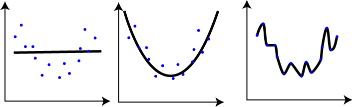
To avoid overfitting, we will first split out data to training set and test set and test out model on the test set.
Next: we will use two of keras's callbacks EarlyStopping and ModelCheckpoint
Let's see first the model we implemented
model.summary()
_________________________________________________________________
Layer (type)                 Output Shape              Param #
=================================================================
dense_1 (Dense)              (None, 1)                 13
=================================================================
Total params: 13
Trainable params: 13
Non-trainable params: 0
_________________________________________________________________
from sklearn.model_selection import train_test_split
from keras.callbacks import EarlyStopping, ModelCheckpoint
X_train, X_val, Y_train, Y_val = train_test_split(X_train, Y_train, test_size=0.15, random_state=42)

fBestModel = 'best_model.h5'
early_stop = EarlyStopping(monitor='val_loss', patience=2, verbose=1)
best_model = ModelCheckpoint(fBestModel, verbose=0, save_best_only=True)

model.fit(X_train, Y_train, validation_data = (X_val, Y_val), epochs=50,
          batch_size=128, verbose=True, callbacks=[best_model, early_stop])
Train on 300 samples, validate on 54 samples
Epoch 1/50
300/300 [==============================] - 0s 36us/step - loss: 29.3639 - val_loss: 20.0013
Epoch 2/50
300/300 [==============================] - 0s 19us/step - loss: 29.1625 - val_loss: 20.7705
Epoch 3/50
300/300 [==============================] - 0s 20us/step - loss: 28.9633 - val_loss: 21.6343
Epoch 00003: early stopping
<keras.callbacks.History at 0x7fe4846439e8>
Multi-Layer Fully Connected Networks

Forward and Backward Propagation

Q: How hard can it be to build a Multi-Layer Fully-Connected Network with keras?
A: It is basically the same, just add more layers!
K.clear_session()
print("Building model...")
model = Sequential()
model.add(Dense(256, input_shape=(dims,),activation='relu'))
model.add(Dense(256,activation='relu'))
model.add(Dense(output_var))
model.add(Activation('relu'))
model.compile(optimizer='sgd', loss='mean_squared_error')
model.summary()
Building model...
_________________________________________________________________
Layer (type)                 Output Shape              Param #
=================================================================
dense_1 (Dense)              (None, 256)               3328
_________________________________________________________________
dense_2 (Dense)              (None, 256)               65792
_________________________________________________________________
dense_3 (Dense)              (None, 1)                 257
_________________________________________________________________
activation_1 (Activation)    (None, 1)                 0
=================================================================
Total params: 69,377
Trainable params: 69,377
Non-trainable params: 0
_________________________________________________________________
model.fit(X_train, Y_train,
          validation_data = (X_val, Y_val),
          epochs=50,
          callbacks=[PlotLossesKeras()])

Mean squared error (cost function):
training   (min:   10.961, max:  661.521, cur:   10.961)
validation (min:   10.649, max:  315.916, cur:   21.782)
<keras.callbacks.History at 0x7fe425cf7278>
What does the cost function behavior mean over the traning in the above plot?
Your Turn!
Hands On - Keras Fully Connected
Take couple of minutes and try to play with the number of layers and the number of parameters in the layers to get the best results.
K.clear_session()
print("Building model...")
model = Sequential()
model.add(Dense(256, input_shape=(dims,),activation='relu'))

# ...
# ...
# Play with it! add as much layers as you want! try and get better results.

model.add(Dense(output_var))
model.add(Activation('relu'))
model.compile(optimizer='sgd', loss='mean_squared_error')
model.summary()
model.fit(X_train, Y_train,
          validation_data = (X_val, Y_val),
          epochs=50,
          callbacks=[PlotLossesKeras()])
Building a question answering system, an image classification model, a Neural Turing Machine, a word2vec embedder or any other model is just as fast. The ideas behind deep learning are simple, so why should their implementation be painful?