E19 - Neural Networks Implementation
It's time to build your first neural network, which will have a hidden layer.
You will learn how to:
- Implement a 2-class classification neural network with a single hidden layer
- Use units with a non-linear activation function, such as tanh
- Compute the cross entropy loss
- Implement forward and backward propagation
19.1 Planar data classification
# Package imports
import numpy as np
import matplotlib.pyplot as plt
import sklearn
import sklearn.datasets
import sklearn.linear_model

%matplotlib inline

np.random.seed(1) # set a seed so that the results are consistent
Function toolbox
# Useful function to deploy your neural network.
def plot_decision_boundary(model, X, y):
    plt.figure(figsize=(15,10))
    # Set min and max values and give it some padding
    x_min, x_max = X[0, :].min() - 1, X[0, :].max() + 1
    y_min, y_max = X[1, :].min() - 1, X[1, :].max() + 1
    h = 0.01
    # Generate a grid of points with distance h between them
    xx, yy = np.meshgrid(np.arange(x_min, x_max, h), np.arange(y_min, y_max, h))
    # Predict the function value for the whole grid
    Z = model(np.c_[xx.ravel(), yy.ravel()])
    Z = Z.reshape(xx.shape)
    # Plot the contour and training examples
    plt.contourf(xx, yy, Z, cmap=plt.cm.Spectral)
    plt.ylabel('x2')
    plt.xlabel('x1')
    plt.scatter(X[0, :], X[1, :], c=y.ravel(), s=80, cmap=plt.cm.Spectral)


def sigmoid(x):
    """
    Compute the sigmoid of x
    Arguments:
    x -- A scalar or numpy array of any size.
    Return:
    s -- sigmoid(x)
    """
    s = 1/(1+np.exp(-x))
    return s

def load_planar_dataset():
    np.random.seed(1)
    m = 400 # number of examples
    N = int(m/2) # number of points per class
    D = 2 # dimensionality
    X = np.zeros((m,D)) # data matrix where each row is a single example
    Y = np.zeros((m,1), dtype='uint8') # labels vector (0 for red, 1 for blue)
    a = 4 # maximum ray of the flower

    for j in range(2):
        ix = range(N*j,N*(j+1))
        t = np.linspace(j*3.12,(j+1)*3.12,N) + np.random.randn(N)*0.2 # theta
        r = a*np.sin(4*t) + np.random.randn(N)*0.2 # radius
        X[ix] = np.c_[r*np.sin(t), r*np.cos(t)]
        Y[ix] = j

    X = X.T
    Y = Y.T

    return X, Y
# These functions will be used to test in a simple way the correctness of the procedure.

def layer_sizes_test_case():
    np.random.seed(1)
    X_assess = np.random.randn(5, 3)
    Y_assess = np.random.randn(2, 3)
    return X_assess, Y_assess

def initialize_parameters_test_case():
    n_x, n_h, n_y = 2, 4, 1
    return n_x, n_h, n_y


def forward_propagation_test_case():
    np.random.seed(1)
    X_assess = np.random.randn(2, 3)
    b1 = np.random.randn(4,1)
    b2 = np.array([[ -1.3]])

    parameters = {'W1': np.array([[-0.00416758, -0.00056267],
        [-0.02136196,  0.01640271],
        [-0.01793436, -0.00841747],
        [ 0.00502881, -0.01245288]]),
     'W2': np.array([[-0.01057952, -0.00909008,  0.00551454,  0.02292208]]),
     'b1': b1,
     'b2': b2}

    return X_assess, parameters

def compute_cost_test_case():
    np.random.seed(1)
    Y_assess = (np.random.randn(1, 3) > 0)
    parameters = {'W1': np.array([[-0.00416758, -0.00056267],
        [-0.02136196,  0.01640271],
        [-0.01793436, -0.00841747],
        [ 0.00502881, -0.01245288]]),
     'W2': np.array([[-0.01057952, -0.00909008,  0.00551454,  0.02292208]]),
     'b1': np.array([[ 0.],
        [ 0.],
        [ 0.],
        [ 0.]]),
     'b2': np.array([[ 0.]])}

    a2 = (np.array([[ 0.5002307 ,  0.49985831,  0.50023963]]))

    return a2, Y_assess, parameters

def backward_propagation_test_case():
    np.random.seed(1)
    X_assess = np.random.randn(2, 3)
    Y_assess = (np.random.randn(1, 3) > 0)
    parameters = {'W1': np.array([[-0.00416758, -0.00056267],
        [-0.02136196,  0.01640271],
        [-0.01793436, -0.00841747],
        [ 0.00502881, -0.01245288]]),
     'W2': np.array([[-0.01057952, -0.00909008,  0.00551454,  0.02292208]]),
     'b1': np.array([[ 0.],
        [ 0.],
        [ 0.],
        [ 0.]]),
     'b2': np.array([[ 0.]])}

    cache = {'A1': np.array([[-0.00616578,  0.0020626 ,  0.00349619],
         [-0.05225116,  0.02725659, -0.02646251],
         [-0.02009721,  0.0036869 ,  0.02883756],
         [ 0.02152675, -0.01385234,  0.02599885]]),
  'A2': np.array([[ 0.5002307 ,  0.49985831,  0.50023963]]),
  'Z1': np.array([[-0.00616586,  0.0020626 ,  0.0034962 ],
         [-0.05229879,  0.02726335, -0.02646869],
         [-0.02009991,  0.00368692,  0.02884556],
         [ 0.02153007, -0.01385322,  0.02600471]]),
  'Z2': np.array([[ 0.00092281, -0.00056678,  0.00095853]])}
    return parameters, cache, X_assess, Y_assess

def update_parameters_test_case():
    parameters = {'W1': np.array([[-0.00615039,  0.0169021 ],
        [-0.02311792,  0.03137121],
        [-0.0169217 , -0.01752545],
        [ 0.00935436, -0.05018221]]),
 'W2': np.array([[-0.0104319 , -0.04019007,  0.01607211,  0.04440255]]),
 'b1': np.array([[ -8.97523455e-07],
        [  8.15562092e-06],
        [  6.04810633e-07],
        [ -2.54560700e-06]]),
 'b2': np.array([[  9.14954378e-05]])}

    grads = {'dW1': np.array([[ 0.00023322, -0.00205423],
        [ 0.00082222, -0.00700776],
        [-0.00031831,  0.0028636 ],
        [-0.00092857,  0.00809933]]),
 'dW2': np.array([[ -1.75740039e-05,   3.70231337e-03,  -1.25683095e-03,
          -2.55715317e-03]]),
 'db1': np.array([[  1.05570087e-07],
        [ -3.81814487e-06],
        [ -1.90155145e-07],
        [  5.46467802e-07]]),
 'db2': np.array([[ -1.08923140e-05]])}
    return parameters, grads

def nn_model_test_case():
    np.random.seed(1)
    X_assess = np.random.randn(2, 3)
    Y_assess = (np.random.randn(1, 3) > 0)
    return X_assess, Y_assess

def predict_test_case():
    np.random.seed(1)
    X_assess = np.random.randn(2, 3)
    parameters = {'W1': np.array([[-0.00615039,  0.0169021 ],
        [-0.02311792,  0.03137121],
        [-0.0169217 , -0.01752545],
        [ 0.00935436, -0.05018221]]),
     'W2': np.array([[-0.0104319 , -0.04019007,  0.01607211,  0.04440255]]),
     'b1': np.array([[ -8.97523455e-07],
        [  8.15562092e-06],
        [  6.04810633e-07],
        [ -2.54560700e-06]]),
     'b2': np.array([[  9.14954378e-05]])}
    return parameters, X_assess
Create Dataset
First, let's get the dataset you will work on. The following code will load a "flower" 2-class dataset into variables X and Y.
X, Y = load_planar_dataset()
Visualize the dataset using matplotlib. The data looks like a "flower" with some red (label y=0) and some blue (y=1) points. Your goal is to build a model to fit this data.
# Visualize the data:
plt.figure(figsize=(15,10))
plt.scatter(X[0, :], X[1, :], c=Y.ravel(), s=40, cmap=plt.cm.Spectral);

You have: - a numpy-array (matrix) X that contains your features (x1, x2) - a numpy-array (vector) Y that contains your labels (red:0, blue:1).
Lets first get a better sense of what our data is like.
Exercise: How many training examples do you have? In addition, what is the shape of the variables X and Y?
Simple Logistic Regression Baseline
Before building a full neural network, lets first see how logistic regression performs on this problem. You can use sklearn's built-in functions to do that. Run the code below to train a logistic regression classifier on the dataset.
# Train the logistic regression classifier
clf = sklearn.linear_model.LogisticRegressionCV(cv=10);
clf.fit(X.T, Y.ravel().T);
You can now plot the decision boundary of these models. Run the code below.
# Plot the decision boundary for logistic regression
plot_decision_boundary(lambda x: clf.predict(x), X, Y)
plt.title("Logistic Regression")
plt.show()
# Print accuracy
LR_predictions = clf.predict(X.T)
print ('Accuracy of logistic regression: %d ' % float((np.dot(Y,LR_predictions) + np.dot(1-Y,1-LR_predictions))/float(Y.size)*100) +
       '% ' + "(percentage of correctly labelled datapoints)")

Accuracy of logistic regression: 46 % (percentage of correctly labelled datapoints)
Exercise: Why is the model performance too low? Explain it with the knowledge you learnt in class.
Neural Network model - MLP
Logistic regression did not work well on the "flower dataset". You are going to train a Neural Network with a single hidden layer.
Here is our model:
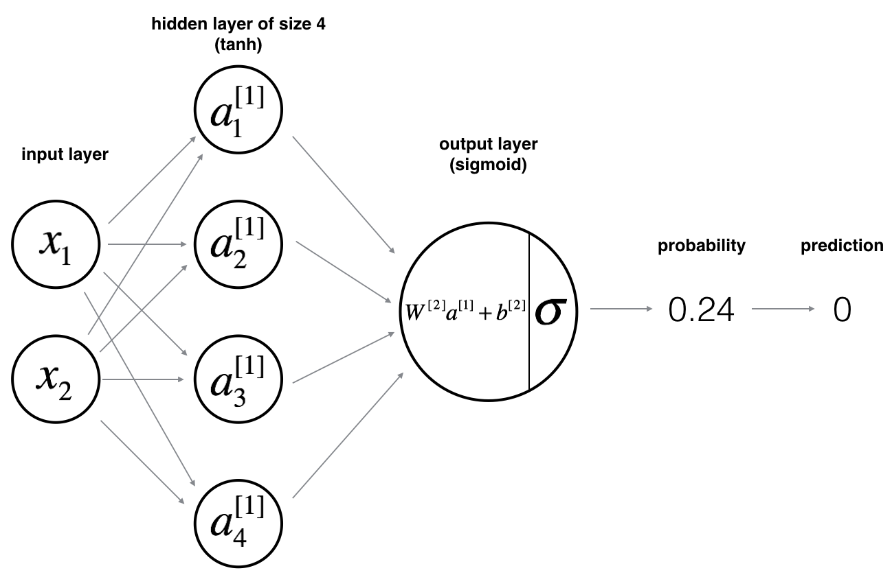
Mathematically:
For one example $x^{(i)}$: $$z^{[1] (i)} = W^{[1]} x^{(i)} + b^{[1]}\tag{1}$$ $$a^{[1] (i)} = \tanh(z^{[1] (i)})\tag{2}$$ $$z^{[2] (i)} = W^{[2]} a^{[1] (i)} + b^{[2]}\tag{3}$$ $$\hat{y}^{(i)} = a^{[2] (i)} = \sigma(z^{ [2] (i)})\tag{4}$$ $$y^{(i)}_{prediction} = \begin{cases} 1 & \mbox{if } a^{[2](i)} > 0.5 \\ 0 & \mbox{otherwise } \end{cases}\tag{5}$$
Given the predictions on all the examples, you can also compute the cost $J$ as follows: $$J = - \frac{1}{m} \sum\limits_{i = 0}^{m} \large\left(\small y^{(i)}\log\left(a^{[2] (i)}\right) + (1-y^{(i)})\log\left(1- a^{[2] (i)}\right) \large \right) \small \tag{6}$$
Reminder: The general methodology to build a Neural Network is to: 1. Define the neural network structure ( # of input units, # of hidden units, etc). 2. Initialize the model's parameters 3. Loop: - Implement forward propagation - Compute loss - Implement backward propagation to get the gradients - Update parameters (gradient descent)
You often build helper functions to compute steps 1-3 and then merge them into one function we call nn_model(). Once you've built nn_model() and learnt the right parameters, you can make predictions on new data.
Defining the neural network structure
Exercise: Define three variables: - n_x: the size of the input layer - n_h: the size of the hidden layer (set this to 4) - n_y: the size of the output layer
Hint: Use shapes of X and Y to find n_x and n_y. Also, hard code the hidden layer size to be 4.
# Solved Exercise

def layer_sizes(X, Y):
    """
    Arguments:
    X -- input dataset of shape (input size, number of examples)
    Y -- labels of shape (output size, number of examples)

    Returns:
    n_x -- the size of the input layer
    n_h -- the size of the hidden layer
    n_y -- the size of the output layer
    """
    ### START CODE HERE ### (≈ 3 lines of code)
    n_x = X.shape[0] # size of input layer
    n_h = 4
    n_y = Y.shape[0] # size of output layer
    ### END CODE HERE ###
    return (n_x, n_h, n_y)
X_assess, Y_assess = layer_sizes_test_case()
(n_x, n_h, n_y) = layer_sizes(X_assess, Y_assess)
print("The size of the input layer is: n_x = " + str(n_x))
print("The size of the hidden layer is: n_h = " + str(n_h))
print("The size of the output layer is: n_y = " + str(n_y))
The size of the input layer is: n_x = 5
The size of the hidden layer is: n_h = 4
The size of the output layer is: n_y = 2
Expected Output (these are not the sizes you will use for your network, they are just used to assess the function you've just coded).
| **n_x** | 5 |
| **n_h** | 4 |
| **n_y** | 2 |
Initialize the model's parameters
Exercise: Implement the function initialize_parameters().
Instructions:
- Make sure your parameters' sizes are right. Refer to the neural network figure above if needed.
- You will initialize the weights matrices with random values.
- Use:
np.random.randn(a,b) * 0.01to randomly initialize a matrix of shape (a,b).
- Use:
- You will initialize the bias vectors as zeros.
- Use:
np.zeros((a,b))to initialize a matrix of shape (a,b) with zeros.
- Use:
# Solved Exercise: initialize_parameters

def initialize_parameters(n_x, n_h, n_y):
    """
    Argument:
    n_x -- size of the input layer
    n_h -- size of the hidden layer
    n_y -- size of the output layer

    Returns:
    params -- python dictionary containing your parameters:
                    W1 -- weight matrix of shape (n_h, n_x)
                    b1 -- bias vector of shape (n_h, 1)
                    W2 -- weight matrix of shape (n_y, n_h)
                    b2 -- bias vector of shape (n_y, 1)
    """

    np.random.seed(2) # we set up a seed so that your output matches ours although the initialization is random.

    ### START CODE HERE ### (≈ 4 lines of code)
    W1 = np.random.randn(n_h,n_x) * 0.01
    b1 = np.zeros(shape=(n_h,1))
    W2 = np.random.randn(n_y,n_h) * 0.01
    b2 = np.zeros(shape=(n_y,1))
    ### END CODE HERE ###

    assert (W1.shape == (n_h, n_x))
    assert (b1.shape == (n_h, 1))
    assert (W2.shape == (n_y, n_h))
    assert (b2.shape == (n_y, 1))

    parameters = {"W1": W1,
                  "b1": b1,
                  "W2": W2,
                  "b2": b2}

    return parameters
n_x, n_h, n_y = initialize_parameters_test_case()

parameters = initialize_parameters(n_x, n_h, n_y)
print("W1 = " + str(parameters["W1"]))
print("b1 = " + str(parameters["b1"]))
print("W2 = " + str(parameters["W2"]))
print("b2 = " + str(parameters["b2"]))
W1 = [[-0.00416758 -0.00056267]
 [-0.02136196  0.01640271]
 [-0.01793436 -0.00841747]
 [ 0.00502881 -0.01245288]]
b1 = [[0.]
 [0.]
 [0.]
 [0.]]
W2 = [[-0.01057952 -0.00909008  0.00551454  0.02292208]]
b2 = [[0.]]
Expected Output:
| **W1** | [[-0.00416758 -0.00056267] [-0.02136196 0.01640271] [-0.01793436 -0.00841747] [ 0.00502881 -0.01245288]] |
| **b1** | [[ 0.] [ 0.] [ 0.] [ 0.]] |
| **W2** | [[-0.01057952 -0.00909008 0.00551454 0.02292208]] |
| **b2** | [[ 0.]] |
The Loop
Question: Implement forward_propagation().
Instructions:
- Look above at the mathematical representation of your classifier.
- You can use the function
sigmoid(). It is built-in (imported) in the notebook. - You can use the function
np.tanh(). It is part of the numpy library. - The steps you have to implement are:
- Retrieve each parameter from the dictionary "parameters" (which is the output of
initialize_parameters()) by usingparameters[".."]. - Implement Forward Propagation. Compute $Z^{[1]}, A^{[1]}, Z^{[2]}$ and $A^{[2]}$ (the vector of all your predictions on all the examples in the training set).
- Retrieve each parameter from the dictionary "parameters" (which is the output of
- Values needed in the backpropagation are stored in "
cache". Thecachewill be given as an input to the backpropagation function.
# Solved Exercise:  forward_propagation

def forward_propagation(X, parameters):
    """
    Argument:
    X -- input data of size (n_x, m)
    parameters -- python dictionary containing your parameters (output of initialization function)

    Returns:
    A2 -- The sigmoid output of the second activation
    cache -- a dictionary containing "Z1", "A1", "Z2" and "A2"
    """
    # Retrieve each parameter from the dictionary "parameters"
    ### START CODE HERE ### (≈ 4 lines of code)
    W1 = parameters["W1"]
    b1 = parameters["b1"]
    W2 = parameters["W2"]
    b2 = parameters["b2"]
    ### END CODE HERE ###

    # Implement Forward Propagation to calculate A2 (probabilities)
    ### START CODE HERE ### (≈ 4 lines of code)
    Z1 = np.dot(W1,X)+b1
    A1 = np.tanh(Z1)
    Z2 = np.dot(W2,A1)+b2
    A2 = sigmoid(Z2)
    ### END CODE HERE ###

    assert(A2.shape == (1, X.shape[1]))

    cache = {"Z1": Z1,
             "A1": A1,
             "Z2": Z2,
             "A2": A2}

    return A2, cache
X_assess, parameters = forward_propagation_test_case()
A2, cache = forward_propagation(X_assess, parameters)

# Note: we use the mean here just to make sure that your output matches ours.
print(np.mean(cache['Z1']) ,np.mean(cache['A1']),np.mean(cache['Z2']),np.mean(cache['A2']))
0.26281864019752443 0.09199904522700113 -1.3076660128732143 0.21287768171914198
Expected Output:
| 0.262818640198 0.091999045227 -1.30766601287 0.212877681719 |
Now that you have computed $A^{[2]}$ (in the Python variable "A2"), which contains $a^{[2](i)}$ for every example, you can compute the cost function as follows:
Exercise: Implement compute_cost() to compute the value of the cost $J$.
Instructions:
- There are many ways to implement the cross-entropy loss. To help you, we give you how we would have implemented
$- \sum\limits_{i=0}^{m} y^{(i)}\log(a^{[2](i)})$:
logprobs = np.multiply(np.log(A2),Y)
cost = - np.sum(logprobs)                # no need to use a for loop!
(you can use either np.multiply() and then np.sum() or directly np.dot()).
# Solved function: compute_cost

def compute_cost(A2, Y, parameters):
    """
    Computes the cross-entropy cost given in equation (13)

    Arguments:
    A2 -- The sigmoid output of the second activation, of shape (1, number of examples)
    Y -- "true" labels vector of shape (1, number of examples)
    parameters -- python dictionary containing your parameters W1, b1, W2 and b2

    Returns:
    cost -- cross-entropy cost given equation (13)
    """

    m = Y.shape[1] # number of example

    # Compute the cross-entropy cost
    ### START CODE HERE ### (≈ 2 lines of code)
    logprobs = np.multiply(Y,np.log(A2)) + np.multiply(1-Y,np.log(1-A2))
    cost = -1/m * np.sum(logprobs)
    ### END CODE HERE ###

    cost = np.squeeze(cost)     # makes sure cost is the dimension we expect.
                                # E.g., turns [[17]] into 17
    assert(isinstance(cost, float))

    return cost
A2, Y_assess, parameters = compute_cost_test_case()

print("cost = " + str(compute_cost(A2, Y_assess, parameters)))
cost = 0.6930587610394646
Expected Output:
| **cost** | 0.693058761... |
Using the cache computed during forward propagation, you can now implement backward propagation.
Question: Implement the function backward_propagation().
Instructions: Backpropagation is usually the hardest (most mathematical) part in deep learning. To help you, here again is the slide from the lecture on backpropagation. You'll want to use the six equations on the right of this slide, since you are building a vectorized implementation.
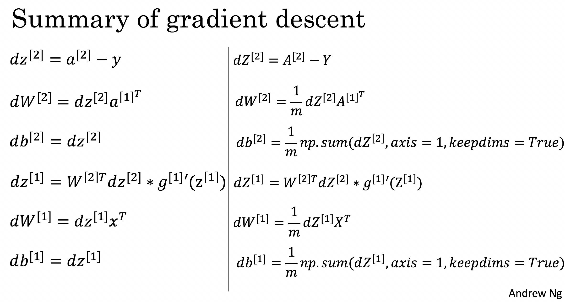
- Tips:
- To compute dZ1 you'll need to compute $g^{[1]'}(Z^{[1]})$. Since $g^{[1]}(.)$ is the tanh activation function, if $a = g^{[1]}(z)$ then $g^{[1]'}(z) = 1-a^2$. So you can compute
(1 - np.power(A1, 2)).
# Solved Function: backward_propagation

def backward_propagation(parameters, cache, X, Y):
    """
    Implement the backward propagation using the instructions above.

    Arguments:
    parameters -- python dictionary containing our parameters
    cache -- a dictionary containing "Z1", "A1", "Z2" and "A2".
    X -- input data of shape (2, number of examples)
    Y -- "true" labels vector of shape (1, number of examples)

    Returns:
    grads -- python dictionary containing your gradients with respect to different parameters
    """
    m = X.shape[1]

    # First, retrieve W1 and W2 from the dictionary "parameters".
    ### START CODE HERE ### (≈ 2 lines of code)
    W1 = parameters["W1"]
    W2 = parameters["W2"]
    ### END CODE HERE ###

    # Retrieve also A1 and A2 from dictionary "cache".
    ### START CODE HERE ### (≈ 2 lines of code)
    A1 = cache["A1"]
    A2 = cache["A2"]
    ### END CODE HERE ###

    # Backward propagation: calculate dW1, db1, dW2, db2.
    ### START CODE HERE ### (≈ 6 lines of code, corresponding to 6 equations on slide above)
    dZ2 = A2 - Y
    dW2 = 1/m * np.dot(dZ2,A1.T)
    db2 = 1/m*np.sum(dZ2,axis=1,keepdims=True)
    dZ1 = np.dot(W2.T,dZ2) * (1 - np.power(A1,2))
    dW1 = 1/m* np.dot(dZ1,X.T)
    db1 = 1/m*np.sum(dZ1,axis=1,keepdims=True)
    ### END CODE HERE ###

    grads = {"dW1": dW1,
             "db1": db1,
             "dW2": dW2,
             "db2": db2}

    return grads
parameters, cache, X_assess, Y_assess = backward_propagation_test_case()

grads = backward_propagation(parameters, cache, X_assess, Y_assess)
print ("dW1 = "+ str(grads["dW1"]))
print ("db1 = "+ str(grads["db1"]))
print ("dW2 = "+ str(grads["dW2"]))
print ("db2 = "+ str(grads["db2"]))
dW1 = [[ 0.00301023 -0.00747267]
 [ 0.00257968 -0.00641288]
 [-0.00156892  0.003893  ]
 [-0.00652037  0.01618243]]
db1 = [[ 0.00176201]
 [ 0.00150995]
 [-0.00091736]
 [-0.00381422]]
dW2 = [[ 0.00078841  0.01765429 -0.00084166 -0.01022527]]
db2 = [[-0.16655712]]
Expected output:
| **dW1** | [[ 0.00301023 -0.00747267] [ 0.00257968 -0.00641288] [-0.00156892 0.003893 ] [-0.00652037 0.01618243]] |
| **db1** | [[ 0.00176201] [ 0.00150995] [-0.00091736] [-0.00381422]] |
| **dW2** | [[ 0.00078841 0.01765429 -0.00084166 -0.01022527]] |
| **db2** | [[-0.16655712]] |
Question: Implement the update rule. Use gradient descent. You have to use (dW1, db1, dW2, db2) in order to update (W1, b1, W2, b2).
General gradient descent rule: $ \theta = \theta - \alpha \frac{\partial J }{ \partial \theta }$ where $\alpha$ is the learning rate and $\theta$ represents a parameter.
Illustration: The gradient descent algorithm with a good learning rate (converging) and a bad learning rate (diverging). Images courtesy of Adam Harley.
# Solved Function :  update_parameters

def update_parameters(parameters, grads, learning_rate = 1.2):
    """
    Updates parameters using the gradient descent update rule given above

    Arguments:
    parameters -- python dictionary containing your parameters
    grads -- python dictionary containing your gradients

    Returns:
    parameters -- python dictionary containing your updated parameters
    """
    # Retrieve each parameter from the dictionary "parameters"
    ### START CODE HERE ### (≈ 4 lines of code)
    W1 = parameters["W1"]
    b1 = parameters["b1"]
    W2 = parameters["W2"]
    b2 = parameters["b2"]
    ### END CODE HERE ###

    # Retrieve each gradient from the dictionary "grads"
    ### START CODE HERE ### (≈ 4 lines of code)
    dW1 = grads["dW1"]
    db1 = grads["db1"]
    dW2 = grads["dW2"]
    db2 = grads["db2"]
    ## END CODE HERE ###

    # Update rule for each parameter
    ### START CODE HERE ### (≈ 4 lines of code)
    W1 = W1 - learning_rate * dW1
    b1 = b1 - learning_rate * db1
    W2 = W2 - learning_rate * dW2
    b2 = b2 - learning_rate * db2
    ### END CODE HERE ###

    parameters = {"W1": W1,
                  "b1": b1,
                  "W2": W2,
                  "b2": b2}

    return parameters
parameters, grads = update_parameters_test_case()
parameters = update_parameters(parameters, grads)

print("W1 = " + str(parameters["W1"]))
print("b1 = " + str(parameters["b1"]))
print("W2 = " + str(parameters["W2"]))
print("b2 = " + str(parameters["b2"]))
W1 = [[-0.00643025  0.01936718]
 [-0.02410458  0.03978052]
 [-0.01653973 -0.02096177]
 [ 0.01046864 -0.05990141]]
b1 = [[-1.02420756e-06]
 [ 1.27373948e-05]
 [ 8.32996807e-07]
 [-3.20136836e-06]]
W2 = [[-0.01041081 -0.04463285  0.01758031  0.04747113]]
b2 = [[0.00010457]]
Expected Output:
| **W1** | [[-0.00643025 0.01936718] [-0.02410458 0.03978052] [-0.01653973 -0.02096177] [ 0.01046864 -0.05990141]] |
| **b1** | [[ -1.02420756e-06] [ 1.27373948e-05] [ 8.32996807e-07] [ -3.20136836e-06]] |
| **W2** | [[-0.01041081 -0.04463285 0.01758031 0.04747113]] |
| **b2** | [[ 0.00010457]] |
Integrate parts [Network structure ,Model Parameters, the loop] in nn_model()
Question: Build your neural network model in nn_model().
Instructions: The neural network model has to use the previous functions in the right order.
# Solved Function: nn_model

def nn_model(X, Y, n_h, num_iterations = 10000, print_cost=False):
    """
    Arguments:
    X -- dataset of shape (2, number of examples)
    Y -- labels of shape (1, number of examples)
    n_h -- size of the hidden layer
    num_iterations -- Number of iterations in gradient descent loop
    print_cost -- if True, print the cost every 1000 iterations

    Returns:
    parameters -- parameters learnt by the model. They can then be used to predict.
    """

    np.random.seed(3)
    n_x = layer_sizes(X, Y)[0]
    n_y = layer_sizes(X, Y)[2]

    # Initialize parameters, then retrieve W1, b1, W2, b2. Inputs: "n_x, n_h, n_y". Outputs = "W1, b1, W2, b2, parameters".
    ### START CODE HERE ### (≈ 5 lines of code)
    parameters = initialize_parameters(n_x,n_h,n_y)
    W1 = parameters["W1"]
    b1 = parameters["b1"]
    W2 = parameters["W2"]
    b2 = parameters["b2"]
    ### END CODE HERE ###

    # Loop (gradient descent)

    for i in range(0, num_iterations):

        ### START CODE HERE ### (≈ 4 lines of code)
        # Forward propagation. Inputs: "X, parameters". Outputs: "A2, cache".
        A2, cache = forward_propagation(X, parameters)

        # Cost function. Inputs: "A2, Y, parameters". Outputs: "cost".
        cost = compute_cost(A2,Y,parameters)

        # Backpropagation. Inputs: "parameters, cache, X, Y". Outputs: "grads".
        grads = backward_propagation(parameters,cache,X,Y)

        # Gradient descent parameter update. Inputs: "parameters, grads". Outputs: "parameters".
        parameters = update_parameters(parameters,grads)

        ### END CODE HERE ###

        # Print the cost every 1000 iterations
        if print_cost and i % 1000 == 0:
            print ("Cost after iteration %i: %f" %(i, cost))

    return parameters
X_assess, Y_assess = nn_model_test_case()
parameters = nn_model(X_assess, Y_assess, 4, num_iterations=10000, print_cost=True)
print("W1 = " + str(parameters["W1"]))
print("b1 = " + str(parameters["b1"]))
print("W2 = " + str(parameters["W2"]))
print("b2 = " + str(parameters["b2"]))
Cost after iteration 0: 0.692739
Cost after iteration 1000: 0.000218
Cost after iteration 2000: 0.000107
Cost after iteration 3000: 0.000071
Cost after iteration 4000: 0.000053
Cost after iteration 5000: 0.000042
Cost after iteration 6000: 0.000035
Cost after iteration 7000: 0.000030
Cost after iteration 8000: 0.000026
Cost after iteration 9000: 0.000023
W1 = [[-0.65848169  1.21866811]
 [-0.76204273  1.39377573]
 [ 0.5792005  -1.10397703]
 [ 0.76773391 -1.41477129]]
b1 = [[ 0.287592  ]
 [ 0.3511264 ]
 [-0.2431246 ]
 [-0.35772805]]
W2 = [[-2.45566237 -3.27042274  2.00784958  3.36773273]]
b2 = [[0.20459656]]
Expected Output:
| **cost after iteration 0** | 0.692739 |
|
|
|
| **W1** | [[-0.65848169 1.21866811] [-0.76204273 1.39377573] [ 0.5792005 -1.10397703] [ 0.76773391 -1.41477129]] |
| **b1** | [[ 0.287592 ] [ 0.3511264 ] [-0.2431246 ] [-0.35772805]] |
| **W2** | [[-2.45566237 -3.27042274 2.00784958 3.36773273]] |
| **b2** | [[ 0.20459656]] |
Predictions
Question: Use your model to predict by building predict(). Use forward propagation to predict results.
Reminder: predictions = $y_{prediction} = \mathbb 1 \text{{activation > 0.5}} = \begin{cases} 1 & \text{if}\ activation > 0.5 \\ 0 & \text{otherwise} \end{cases}$
As an example, if you would like to set the entries of a matrix X to 0 and 1 based on a threshold you would do: X_new = (X > threshold)
# Solved Function: predict

def predict(parameters, X):
    """
    Using the learned parameters, predicts a class for each example in X

    Arguments:
    parameters -- python dictionary containing your parameters
    X -- input data of size (n_x, m)

    Returns
    predictions -- vector of predictions of our model (red: 0 / blue: 1)
    """

    # Computes probabilities using forward propagation, and classifies to 0/1 using 0.5 as the threshold.
    ### START CODE HERE ### (≈ 2 lines of code)
    A2, cache = forward_propagation(X,parameters)
    predictions = A2 > 0.5
    ### END CODE HERE ###

    return predictions
parameters, X_assess = predict_test_case()

predictions = predict(parameters, X_assess)
print("predictions mean = " + str(np.mean(predictions)))
predictions mean = 0.6666666666666666
Expected Output:
| **predictions mean** | 0.666666666667 |
It is time to run the model and see how it performs on a planar dataset. Run the following code to test your model with a single hidden layer of $n_h$ hidden units.
# Build a model with a n_h-dimensional hidden layer
parameters = nn_model(X, Y, n_h = 4, num_iterations = 10000, print_cost=True)

# Plot the decision boundary
plot_decision_boundary(lambda x: predict(parameters, x.T), X, Y)
plt.title("Decision Boundary for hidden layer size " + str(4))
Cost after iteration 0: 0.693048
Cost after iteration 1000: 0.288083
Cost after iteration 2000: 0.254385
Cost after iteration 3000: 0.233864
Cost after iteration 4000: 0.226792
Cost after iteration 5000: 0.222644
Cost after iteration 6000: 0.219731
Cost after iteration 7000: 0.217504
Cost after iteration 8000: 0.219467
Cost after iteration 9000: 0.218561
Text(0.5, 1.0, 'Decision Boundary for hidden layer size 4')

Expected Output:
| **Cost after iteration 9000** | 0.218607 |
# Print accuracy
predictions = predict(parameters, X)
print ('Accuracy: %d' % float((np.dot(Y,predictions.T) + np.dot(1-Y,1-predictions.T))/float(Y.size)*100) + '%')
Accuracy: 90%
Expected Output:
| **Accuracy** | 90% |
Accuracy is really high compared to Logistic Regression. The model has learnt the leaf patterns of the flower! Neural networks are able to learn even highly non-linear decision boundaries, unlike logistic regression.
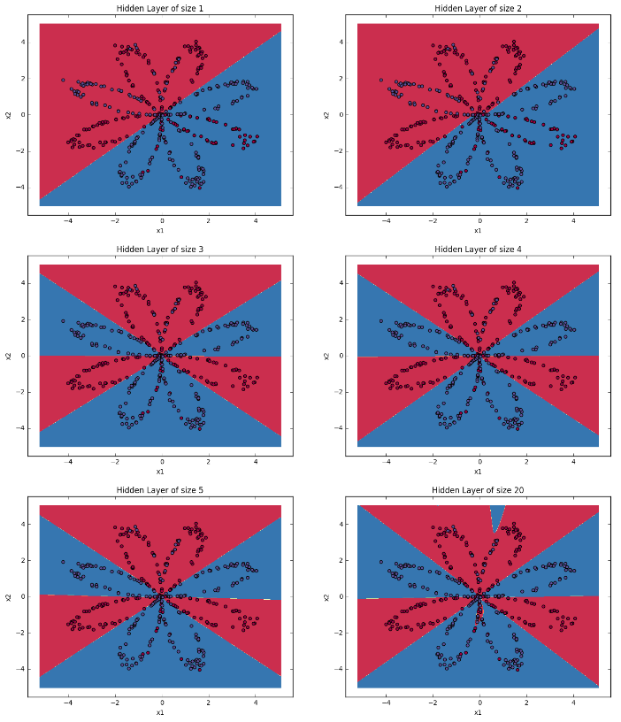
19.2 Tunning hidden layer size
Exercise: Iterate over the number of hidden neurons and report the accuracy and boundary decision plot. Expected results are as follows(Include plots and accuracy).
19.2 Moons Dataset
Replicate the planar points model and report your best accuracy and decision boundary
from sklearn.datasets.samples_generator import make_moons

x_train, y_train = make_moons(n_samples=1000, noise= 0.2, random_state=3)
plt.figure(figsize=(15, 10))
plt.scatter(x_train[:, 0], x_train[:,1], c=y_train, s=40, cmap=plt.cm.Spectral);
