2. Statistical Learning
Excercises from Chapter 2 of An Introduction to Statistical Learning by Gareth James, Daniela Witten, Trevor Hastie and Robert Tibshirani.
I've elected to use Python instead of R.
Conceptual
Q1
For each of parts (a) through (d), indicate whether we would generally expect the performance of a flexible statistical learning method to be better or worse than an inflexible method. Justify your answer.
a) The sample size n is extremely large, and the number of predictors p is small.
Flexible: we have enough observations to avoid overfitting, so assuming some there are non-linear relationships in our data a more flexible model should provide an improved fit.
b) The number of predictors p is extremely large, and the number of observations n is small.
Inflexible: we don't have enough observations to avoid overfitting
c) The relationship between the predictors and response is highly non-linear.
Flexible: a high variance model affords a better fit to non-linear relationships
d) The variance of the error terms, i.e. σ2 = Var(ε), is extremely high.
Inflexible: a high bias model avoids overfitting to the noise in our dataset
Q2
Explain whether each scenario is a classification or regression problem, and indicate whether we are most interested in inference or prediction. Finally, provide n and p.
(a) We collect a set of data on the top 500 firms in the US. For each firm we record profit, number of employees, industry and the CEO salary. We are interested in understanding which factors affect CEO salary.
regression, inference, n=500, p=4
(b) We are considering launching a new product and wish to know whether it will be a success or a failure. We collect data on 20 similar products that were previously launched. For each product we have recorded whether it was a success or failure, price charged for the product, marketing budget, competition price, and ten other variables.
classification, prediction, n=20, p=14
(c) We are interested in predicting the % change in the USD/Euro exchange rate in relation to the weekly changes in the world stock markets. Hence we collect weekly data for all of 2012. For each week we record the % change in the USD/Euro, the % change in the US market, the % change in the British market, and the % change in the German market.
regression, prediction, n=52, p=4
Q3
We now revisit the bias-variance decomposition.
(a) Provide a sketch of typical (squared) bias, variance, training error, test error, and Bayes (or irreducible) error curves, on a single plot, as we go from less flexible statistical learning methods towards more flexible approaches. The x-axis should represent the amount of flexibility in the method, and the y-axis should represent the values for each curve. There should be five curves. Make sure to label each one.
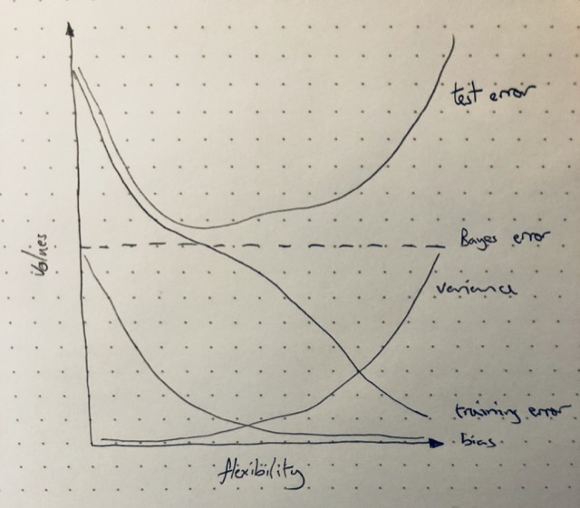
(b) Explain why each of the five curves has the shape displayed in part (a).
- Bayes error: the irreducible error which is a constant irrespective of model flexibility
- Variance: the variance of a model increases with flexibility as the model picks up variation between training sets rsulting in more variaiton in f(X)
- Bias: bias tends to decrease with flexibility as the model casn fit more complex relationships
- Test error: tends to decreases as reduced bias allows the model to better fit non-linear relationships but then increases as an increasingly flexible model begins to fit the noise in the dataset (overfitting)
- Training error: decreases monotonically with increaed flexibility as the model 'flexes' towards individual datapoints in the training set
Q4
You will now think of some real-life applications for statistical learning
(a) Describe three real-life applications in which classification might be useful. Describe the response, as well as the predictors. Is the goal of each application inference or prediction? Explain your answer.
- Is this tumor malignant or benign?
- response: boolean (is malign)
- predictors (naive examples): tumor size, white blood cell count, change in adrenal mass, position in body
- goal: prediction
- What animals are in this image?
- response: 'Cat', 'Dog', 'Fish'
- predictors: image pixel values
- goal: prediction
- What test bench metrics are most indicative of a faulty Printed Circuit Board (PCB)?
- response: boolean (is faulty)
- predictors: current draw, voltage drawer, output noise, operating temp.
- goal: inference
(b) Describe three real-life applications in which regression might be useful. Describe the response, as well as the predictors. Is the goal of each application inference or prediction? Explain your answer.
- How much is this house worth?
- responce: SalePrice
- predictors: LivingArea, BathroomCount, GarageCount, Neighbourhood, CrimeRate
- goal: prediction
- What attributes most affect the market cap. of a company?
- response: MarketCap
- predictors: Sector, Employees, FounderIsCEO, Age, TotalInvestment, Profitability, RONA
- goal: inference
- How long is this dairy cow likely to live?
- response: years
- predictors: past medical conditions, current weight, milk yield
- goal: prediction
(c) Describe three real-life applications in which cluster analysis might be useful.
- This dataset contains observations of 3 different species of flower. Estimate which observations belong to the same species.
- response: a, b, c (species class)
- predictors: sepal length, petal length, number of petals
- goal: prediction
- which attributes of the flowers in dataset described above are most predictive of species?
- response: a, b, c (species class)
- predictors: sepal length, petal length, number of petals
- goal: inference
- Group these audio recordings of birdsong by species.
- responce: (species classes)
- predictors: audio sample values
- goal: prediction
Q5
What are the advantages and disadvantages of a very flexible (versus a less flexible) approach for regression or classification? Under what circumstances might a more flexible approach be preferred to a less flexible approach? When might a less flexible approach be preferred?
Less flexible
- (+) gives better results with few observations
- (+) simpler inference: the effect of each feature can be more easily understood
- (+) fewer parameters, faster optimisation
- (-) performs poorly if observations contain highly non-linear relationships
More flexible
- (+) gives better fit if observations contain non-linear relationships
- (-) can overfit the data providing poor predictions for new observations
Q6
Describe the differences between a parametric and a non-parametric statistical learning approach. What are the advantages of a parametric approach to regression or classification (as opposed to a non-parametric approach)? What are its disadvantages?
A parametric approach simplifies the problem of estimating the best fit to the training data f(x) by making some assumptions about the functional form of f(x), this reduces the problem to estimating the parameters of the model. A non-parametric approach make no such assumptions and so f(x) can take any arbitrary shape.
The advantage of the parametric approach is that it simplifies the problem of estimating f(x) because it is easier to estimate paramters than an arbitrary function. The disadvantage of this approach is that the assumed form of the function f(X) could limit the degree of accuracy with which the model can fit the training data. If too many parameters are used, in an attempt to increase the models flexibility, then overfitting can occur – meaning that the model begins to fit noise in the training data that is not representive of unseen observations.
import numpy as np
import pandas as pd
import seaborn as sns
import warnings
warnings.filterwarnings('ignore')
Q7
The table below provides a training data set containing six observations, three predictors, and one qualitative response variable.
df = pd.DataFrame({'Obs': [1, 2, 3, 4, 5, 6],
                   'X1': [0, 2, 0, 0, -1, 1],
                   'X2': [3, 0, 1, 1, 0, -1],
                   'X3': [0, 0, 3, 2, 1, 1],
                   'Y': ['Red', 'Red', 'Red', 'Green', 'Green', 'Red']})

df
| Obs | X1 | X2 | X3 | Y | |
|---|---|---|---|---|---|
| 0 | 1 | 0 | 3 | 0 | Red |
| 1 | 2 | 2 | 0 | 0 | Red |
| 2 | 3 | 0 | 1 | 3 | Red |
| 3 | 4 | 0 | 1 | 2 | Green |
| 4 | 5 | -1 | 0 | 1 | Green |
| 5 | 6 | 1 | -1 | 1 | Red |
Suppose we wish to use this data set to make a prediction for Y when X1 = X2 = X3 = 0 using K-nearest neighbors.
# (a) Compute the Euclidean distance between each observation and the test point,X1 =X2 =X3 =0.

def euclidian_dist(x):
    """Compute the row-wise euclidean distance
    from the origin"""
    return (np.sum(x**2, axis=1))**0.5

euc_dist = pd.DataFrame({'EuclideanDist': euclidian_dist(df[['X1', 'X2', 'X3']])})
df_euc = pd.concat([df, euc_dist], axis=1)
df_euc
| Obs | X1 | X2 | X3 | Y | EuclideanDist | |
|---|---|---|---|---|---|---|
| 0 | 1 | 0 | 3 | 0 | Red | 3.000000 |
| 1 | 2 | 2 | 0 | 0 | Red | 2.000000 |
| 2 | 3 | 0 | 1 | 3 | Red | 3.162278 |
| 3 | 4 | 0 | 1 | 2 | Green | 2.236068 |
| 4 | 5 | -1 | 0 | 1 | Green | 1.414214 |
| 5 | 6 | 1 | -1 | 1 | Red | 1.732051 |
# (b) What is our prediction with K = 1? Why?

K = 1
df_euc.nsmallest(K, 'EuclideanDist')

# Our prediction is Y=Green because that is the response value of the
# first nearest neighbour to the point X1 = X2 = X3 = 0
| Obs | X1 | X2 | X3 | Y | EuclideanDist | |
|---|---|---|---|---|---|---|
| 4 | 5 | -1 | 0 | 1 | Green | 1.414214 |
# (c) What is our prediction with K = 3? Why?

K = 3
df_euc.nsmallest(K, 'EuclideanDist')

# Red, because majority of the 3 nearest neighbours are Red.
| Obs | X1 | X2 | X3 | Y | EuclideanDist | |
|---|---|---|---|---|---|---|
| 4 | 5 | -1 | 0 | 1 | Green | 1.414214 |
| 5 | 6 | 1 | -1 | 1 | Red | 1.732051 |
| 1 | 2 | 2 | 0 | 0 | Red | 2.000000 |
(d) If the Bayes decision boundary in this problem is highly non-linear, then would we expect the best value for K to be large or small? Why?
Small. A smaller value of K results in a more flexible classification model because the prediciton is based upon a smaller subset of all observations in the dataset.