A Brief History of Perceptrons
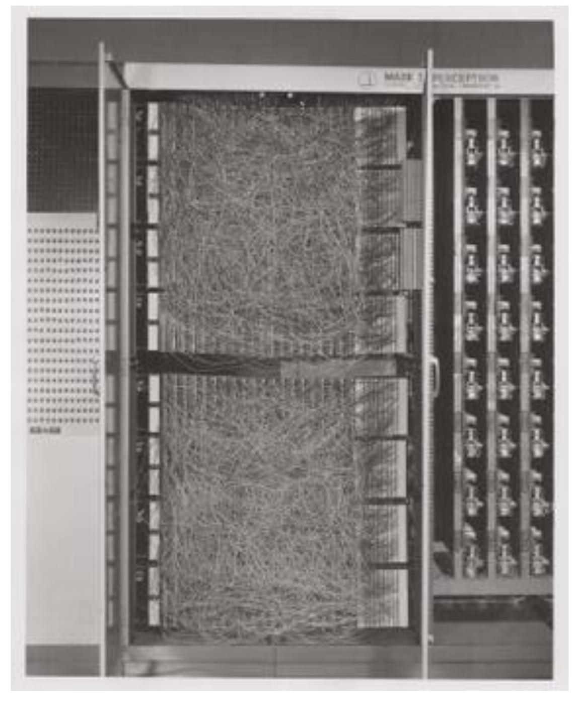
Frank Rosenblatt, godfather of the perceptron, popularized it as a device rather than an algorithm. The perceptron first entered the world as hardware.1 Rosenblatt, a psychologist who studied and later lectured at Cornell University, received funding from the U.S. Office of Naval Research to build a machine that could learn. His machine, the Mark I perceptron, looked like this.
A perceptron is a linear classifier; that is, it is an algorithm that classifies input by separating two categories with a straight line.Rosenblatt built a single-layer perceptron. That is, his hardware-algorithm did not include multiple layers, which allow neural networks to model a feature hierarchy. It was, therefore, a shallow neural network, which prevented his perceptron from performing non-linear classification, such as the XOR function (an XOR operator trigger when input exhibits either one trait or another, but not both; it stands for “exclusive OR”), as Minsky and Papert showed in their book.
Multilayer Perceptron Layer
Subsequent work with multilayer perceptrons has shown that they are capable of approximating an XOR operator as well as many other non-linear functions.
A multilayer perceptron (MLP) is a deep, artificial neural network. It is composed of more than one perceptron. They are composed of an input layer to receive the signal, an output layer that makes a decision or prediction about the input, and in between those two, an arbitrary number of hidden layers that are the true computational engine of the MLP. MLPs with one hidden layer are capable of approximating any continuous function.
Multilayer perceptrons are often applied to supervised learning problems3: they train on a set of input-output pairs and learn to model the correlation (or dependencies) between those inputs and outputs. Training involves adjusting the parameters, or the weights and biases, of the model in order to minimize error. Backpropagation is used to make those weigh and bias adjustments relative to the error, and the error itself can be measured in a variety of ways, including by root mean squared error (RMSE).
import numpy as np
import tensorflow as tf
# Parameters
learning_rate = 0.001
training_steps = 3000
batch_size = 100
display_step = 300
(x_train, y_train), (x_test, y_test) = tf.keras.datasets.mnist.load_data()
# Convert to float32.
x_train, x_test = np.array(x_train, np.float32), np.array(x_test, np.float32)
# Flatten images to 1-D vector of 784 features (28*28).
x_train, x_test = x_train.reshape([-1, 784]), x_test.reshape([-1, 784])
# Normalize images value from [0, 255] to [0, 1].
x_train, x_test = x_train / 255., x_test / 255.

# Use tf.data API to shuffle and batch data.
train_data = tf.data.Dataset.from_tensor_slices((x_train, y_train))
train_data = train_data.repeat().shuffle(5000).batch(batch_size).prefetch(1)
# Network Parameters
n_hidden_1 = 256 # 1st layer number of neurons
n_hidden_2 = 256 # 2nd layer number of neurons
n_input = 784 # MNIST data input (img shape: 28*28)
n_classes = 10 # MNIST total classes (0-9 digits)
# Store layers weight & bias
weights = {
    'h1': tf.Variable(tf.random.normal([n_input, n_hidden_1])),
    'h2': tf.Variable(tf.random.normal([n_hidden_1, n_hidden_2])),
    'out': tf.Variable(tf.random.normal([n_hidden_2, n_classes]))
}
biases = {
    'b1': tf.Variable(tf.random.normal([n_hidden_1])),
    'b2': tf.Variable(tf.random.normal([n_hidden_2])),
    'out': tf.Variable(tf.random.normal([n_classes]))
}
# Create model
def multilayer_perceptron(x):
    # Hidden fully connected layer with 256 neurons
    layer_1 = tf.add(tf.matmul(x, weights['h1']), biases['b1'])
    layer_1 = tf.nn.sigmoid(layer_1)
    # Hidden fully connected layer with 256 neurons
    layer_2 = tf.add(tf.matmul(layer_1, weights['h2']), biases['b2'])
    # Output fully connected layer with a neuron for each class
    layer_2 = tf.nn.sigmoid(layer_2)
    output = tf.matmul(layer_2, weights['out']) + biases['out']
    return tf.nn.softmax(output)

# Cross-Entropy loss function.
def cross_entropy(y_pred, y_true):
    # Encode label to a one hot vector.
    y_true = tf.one_hot(y_true, depth=10)
    # Clip prediction values to avoid log(0) error.
    y_pred = tf.clip_by_value(y_pred, 1e-9, 1.)
    # Compute cross-entropy.
    return tf.reduce_mean(-tf.reduce_sum(y_true * tf.math.log(y_pred)))

# Accuracy metric.
def accuracy(y_pred, y_true):
    # Predicted class is the index of highest score in prediction vector (i.e. argmax).
    correct_prediction = tf.equal(tf.argmax(y_pred, 1), tf.cast(y_true, tf.int64))
    return tf.reduce_mean(tf.cast(correct_prediction, tf.float32), axis=-1)

# Stochastic gradient descent optimizer.
optimizer = tf.optimizers.SGD(learning_rate)
# Optimization process.
def train_step(x, y):
    # Wrap computation inside a GradientTape for automatic differentiation.
    with tf.GradientTape() as tape:
        pred = multilayer_perceptron(x)
        loss = cross_entropy(pred, y)

    # Variables to update, i.e. trainable variables.
    trainable_variables = list(weights.values()) + list(biases.values())

    # Compute gradients.
    gradients = tape.gradient(loss, trainable_variables)

    # Update W and b following gradients.
    optimizer.apply_gradients(zip(gradients, trainable_variables))
# Run training for the given number of steps.
for step, (batch_x, batch_y) in enumerate(train_data.take(training_steps), 1):
    # Run the optimization to update W and b values.
    train_step(batch_x, batch_y)

    if (step+1) % display_step == 0:
        pred = multilayer_perceptron(batch_x)
        loss  = cross_entropy(pred, batch_y)
        acc  = accuracy(pred, batch_y)
        print("step: %i, loss: %f, accuracy: %f" % (step+1, loss, acc))
step: 300, loss: 77.175262, accuracy: 0.770000
step: 600, loss: 69.724609, accuracy: 0.780000
step: 900, loss: 67.467102, accuracy: 0.810000
step: 1200, loss: 34.210907, accuracy: 0.890000
step: 1500, loss: 48.025967, accuracy: 0.860000
step: 1800, loss: 51.137367, accuracy: 0.880000
step: 2100, loss: 62.240646, accuracy: 0.800000
step: 2400, loss: 37.719868, accuracy: 0.880000
step: 2700, loss: 30.107677, accuracy: 0.870000
step: 3000, loss: 28.086235, accuracy: 0.900000