Data analysis in Python
Lesson preamble
Learning objectives
- Describe what a data frame is.
- Load external data from a .csv file into a data frame with pandas.
- Summarize the contents of a data frame with pandas.
- Learn to use data frame attributes
loc[],head(),info(),describe(),shape,columns,index. - Learn to clean dirty data.
- Understand the split-apply-combine concept for data analysis.
- Use
groupby(),mean(),agg()andsize()to apply this technique.
- Use
Lesson outline
- Manipulating and analyzing data with pandas
- Data set background (10 min)
- What are data frames (15 min)
- Data wrangling with pandas (40 min)
- Cleaning data (20 min)
- Split-apply-combine techniques in
pandas- Using
mean()to summarize categorical data (20 min) - Using
size()to summarize categorical data (15 min)
- Using
Manipulating and analyzing data with pandas
Dataset background
Today, we will be working with real data about the world combined from multiple sources by the Gapminder foundation. Gapminder is and independent Swedish foundation that fights devastating misconceptions about global development and promotes as fact-based world view through the production of free teaching and data exploration resources. Insights from the combined Gapminder data sources have been popularized through the efforts of public health professor Hans Rosling, and it is highly recommended to check out his entertaining videos, for example this one.
As a start, we recommend taking this 5-10 min quiz to see how ignorant you are about the world. Then we will learn how to dive into this data further using Python!
Overview of the gapminder world data
We are studying the species and weight of animals caught in plots in our study area. The dataset is stored as a comma separated value (CSV) file. Each row holds information for a single animal, and the columns represent:
| Column | Description |
|---|---|
| country | Country name |
| year | Year of observation |
| population | Population in the country at each year |
| region | Continent the country belongs to |
| sub_region | Sub regions as defined by |
| income_group | Income group as specified by the world bank |
| life_expectancy | The average number of years a newborn child would live if mortality patterns were to stay the same |
| income | GDP per capita (in USD) adjusted for differences in purchasing power |
| children_per_woman | Number of children born to each woman |
| child_mortality | Deaths of children under 5 years |
| pop_density | Average number of people per km2 |
| co2_per_capita | CO2 emissions from fossil fuels (tonnes per capita) |
| years_in_school_men | Average number of years attending primary, secondary, and tertiary school for 25-36 years old men |
| years_in_school_women | Average number of years attending primary, secondary, and tertiary school for 25-36 years old women |
To read the data into Python, we are going to use a function called read_csv from the Python-package pandas. As mentioned previously, Python-packages are a bit like browser extensions, they are not essential, but can provide nifty functionality. To use a package, it first needs to be imported.
# pandas is given the nickname `pd`
import pandas as pd
pandas can read CSV-files saved on the computer or directly from an URL.
world_data = pd.read_csv('https://raw.githubusercontent.com/UofTCoders/2018-09-10-utoronto/gh-pages/data/world-data-gapminder.csv')
To view the result, type world_data in a cell and run it, just as when viewing the content of any variable in Python.
world_data
| country | year | population | region | sub_region | income_group | life_expectancy | income | children_per_woman | child_mortality | pop_density | co2_per_capita | years_in_school_men | years_in_school_women | |
|---|---|---|---|---|---|---|---|---|---|---|---|---|---|---|
| 0 | Afghanistan | 1800 | 3280000 | Asia | Southern Asia | Low | 28.2 | 603 | 7.00 | 469.0 | NaN | NaN | NaN | NaN |
| 1 | Afghanistan | 1801 | 3280000 | Asia | Southern Asia | Low | 28.2 | 603 | 7.00 | 469.0 | NaN | NaN | NaN | NaN |
| 2 | Afghanistan | 1802 | 3280000 | Asia | Southern Asia | Low | 28.2 | 603 | 7.00 | 469.0 | NaN | NaN | NaN | NaN |
| 3 | Afghanistan | 1803 | 3280000 | Asia | Southern Asia | Low | 28.2 | 603 | 7.00 | 469.0 | NaN | NaN | NaN | NaN |
| 4 | Afghanistan | 1804 | 3280000 | Asia | Southern Asia | Low | 28.2 | 603 | 7.00 | 469.0 | NaN | NaN | NaN | NaN |
| 5 | Afghanistan | 1805 | 3280000 | Asia | Southern Asia | Low | 28.2 | 603 | 7.00 | 469.0 | NaN | NaN | NaN | NaN |
| 6 | Afghanistan | 1806 | 3280000 | Asia | Southern Asia | Low | 28.1 | 603 | 7.00 | 470.0 | NaN | NaN | NaN | NaN |
| 7 | Afghanistan | 1807 | 3280000 | Asia | Southern Asia | Low | 28.1 | 603 | 7.00 | 470.0 | NaN | NaN | NaN | NaN |
| 8 | Afghanistan | 1808 | 3280000 | Asia | Southern Asia | Low | 28.1 | 603 | 7.00 | 470.0 | NaN | NaN | NaN | NaN |
| 9 | Afghanistan | 1809 | 3280000 | Asia | Southern Asia | Low | 28.1 | 603 | 7.00 | 470.0 | NaN | NaN | NaN | NaN |
| 10 | Afghanistan | 1810 | 3280000 | Asia | Southern Asia | Low | 28.1 | 604 | 7.00 | 470.0 | NaN | NaN | NaN | NaN |
| 11 | Afghanistan | 1811 | 3280000 | Asia | Southern Asia | Low | 28.1 | 604 | 7.00 | 470.0 | NaN | NaN | NaN | NaN |
| 12 | Afghanistan | 1812 | 3280000 | Asia | Southern Asia | Low | 28.1 | 604 | 7.00 | 470.0 | NaN | NaN | NaN | NaN |
| 13 | Afghanistan | 1813 | 3280000 | Asia | Southern Asia | Low | 28.1 | 604 | 7.00 | 470.0 | NaN | NaN | NaN | NaN |
| 14 | Afghanistan | 1814 | 3290000 | Asia | Southern Asia | Low | 28.1 | 604 | 7.00 | 470.0 | NaN | NaN | NaN | NaN |
| 15 | Afghanistan | 1815 | 3290000 | Asia | Southern Asia | Low | 28.1 | 604 | 7.00 | 470.0 | NaN | NaN | NaN | NaN |
| 16 | Afghanistan | 1816 | 3300000 | Asia | Southern Asia | Low | 28.1 | 604 | 7.00 | 471.0 | NaN | NaN | NaN | NaN |
| 17 | Afghanistan | 1817 | 3300000 | Asia | Southern Asia | Low | 28.0 | 604 | 7.00 | 471.0 | NaN | NaN | NaN | NaN |
| 18 | Afghanistan | 1818 | 3310000 | Asia | Southern Asia | Low | 28.0 | 604 | 7.00 | 471.0 | NaN | NaN | NaN | NaN |
| 19 | Afghanistan | 1819 | 3320000 | Asia | Southern Asia | Low | 28.0 | 604 | 7.00 | 471.0 | NaN | NaN | NaN | NaN |
| 20 | Afghanistan | 1820 | 3320000 | Asia | Southern Asia | Low | 28.0 | 604 | 7.00 | 471.0 | NaN | NaN | NaN | NaN |
| 21 | Afghanistan | 1821 | 3330000 | Asia | Southern Asia | Low | 28.0 | 607 | 7.00 | 471.0 | NaN | NaN | NaN | NaN |
| 22 | Afghanistan | 1822 | 3340000 | Asia | Southern Asia | Low | 28.0 | 609 | 7.00 | 471.0 | NaN | NaN | NaN | NaN |
| 23 | Afghanistan | 1823 | 3350000 | Asia | Southern Asia | Low | 28.0 | 611 | 7.00 | 471.0 | NaN | NaN | NaN | NaN |
| 24 | Afghanistan | 1824 | 3360000 | Asia | Southern Asia | Low | 28.0 | 613 | 7.00 | 471.0 | NaN | NaN | NaN | NaN |
| 25 | Afghanistan | 1825 | 3380000 | Asia | Southern Asia | Low | 27.9 | 615 | 7.00 | 471.0 | NaN | NaN | NaN | NaN |
| 26 | Afghanistan | 1826 | 3390000 | Asia | Southern Asia | Low | 27.9 | 617 | 7.00 | 473.0 | NaN | NaN | NaN | NaN |
| 27 | Afghanistan | 1827 | 3400000 | Asia | Southern Asia | Low | 27.9 | 619 | 7.00 | 473.0 | NaN | NaN | NaN | NaN |
| 28 | Afghanistan | 1828 | 3420000 | Asia | Southern Asia | Low | 27.9 | 621 | 7.00 | 473.0 | NaN | NaN | NaN | NaN |
| 29 | Afghanistan | 1829 | 3430000 | Asia | Southern Asia | Low | 27.9 | 623 | 7.00 | 473.0 | NaN | NaN | NaN | NaN |
| ... | ... | ... | ... | ... | ... | ... | ... | ... | ... | ... | ... | ... | ... | ... |
| 38952 | Zimbabwe | 1989 | 9900000 | Africa | Sub-Saharan Africa | Low | 62.7 | 2490 | 5.37 | 73.9 | 25.6 | 1.630 | 7.61 | 6.01 |
| 38953 | Zimbabwe | 1990 | 10200000 | Africa | Sub-Saharan Africa | Low | 61.7 | 2590 | 5.18 | 75.2 | 26.3 | 1.540 | 7.74 | 6.16 |
| 38954 | Zimbabwe | 1991 | 10400000 | Africa | Sub-Saharan Africa | Low | 61.0 | 2670 | 5.00 | 77.4 | 27.0 | 1.530 | 7.88 | 6.31 |
| 38955 | Zimbabwe | 1992 | 10700000 | Africa | Sub-Saharan Africa | Low | 59.4 | 2370 | 4.84 | 80.2 | 27.6 | 1.590 | 8.01 | 6.46 |
| 38956 | Zimbabwe | 1993 | 10900000 | Africa | Sub-Saharan Africa | Low | 57.6 | 2350 | 4.69 | 83.4 | 28.2 | 1.500 | 8.14 | 6.61 |
| 38957 | Zimbabwe | 1994 | 11100000 | Africa | Sub-Saharan Africa | Low | 55.8 | 2520 | 4.56 | 86.8 | 28.7 | 1.600 | 8.28 | 6.76 |
| 38958 | Zimbabwe | 1995 | 11300000 | Africa | Sub-Saharan Africa | Low | 53.7 | 2480 | 4.43 | 90.1 | 29.3 | 1.340 | 8.41 | 6.92 |
| 38959 | Zimbabwe | 1996 | 11500000 | Africa | Sub-Saharan Africa | Low | 52.2 | 2690 | 4.33 | 92.8 | 29.8 | 1.300 | 8.54 | 7.07 |
| 38960 | Zimbabwe | 1997 | 11700000 | Africa | Sub-Saharan Africa | Low | 50.8 | 2710 | 4.24 | 94.7 | 30.3 | 1.230 | 8.67 | 7.23 |
| 38961 | Zimbabwe | 1998 | 11900000 | Africa | Sub-Saharan Africa | Low | 49.1 | 2750 | 4.16 | 95.9 | 30.7 | 1.200 | 8.80 | 7.39 |
| 38962 | Zimbabwe | 1999 | 12100000 | Africa | Sub-Saharan Africa | Low | 47.8 | 2690 | 4.10 | 96.4 | 31.2 | 1.310 | 8.93 | 7.55 |
| 38963 | Zimbabwe | 2000 | 12200000 | Africa | Sub-Saharan Africa | Low | 46.7 | 2570 | 4.06 | 96.8 | 31.6 | 1.140 | 9.07 | 7.71 |
| 38964 | Zimbabwe | 2001 | 12400000 | Africa | Sub-Saharan Africa | Low | 46.2 | 2580 | 4.02 | 97.1 | 32.0 | 1.020 | 9.20 | 7.87 |
| 38965 | Zimbabwe | 2002 | 12500000 | Africa | Sub-Saharan Africa | Low | 45.6 | 2320 | 4.00 | 97.7 | 32.3 | 0.957 | 9.33 | 8.03 |
| 38966 | Zimbabwe | 2003 | 12600000 | Africa | Sub-Saharan Africa | Low | 45.3 | 1910 | 3.99 | 98.2 | 32.7 | 0.843 | 9.47 | 8.20 |
| 38967 | Zimbabwe | 2004 | 12800000 | Africa | Sub-Saharan Africa | Low | 45.1 | 1780 | 3.98 | 99.0 | 33.0 | 0.742 | 9.60 | 8.36 |
| 38968 | Zimbabwe | 2005 | 12900000 | Africa | Sub-Saharan Africa | Low | 45.3 | 1650 | 3.99 | 99.7 | 33.4 | 0.832 | 9.73 | 8.53 |
| 38969 | Zimbabwe | 2006 | 13100000 | Africa | Sub-Saharan Africa | Low | 45.7 | 1580 | 3.99 | 100.0 | 33.9 | 0.796 | 9.87 | 8.69 |
| 38970 | Zimbabwe | 2007 | 13300000 | Africa | Sub-Saharan Africa | Low | 46.4 | 1490 | 4.00 | 100.0 | 34.5 | 0.742 | 10.00 | 8.86 |
| 38971 | Zimbabwe | 2008 | 13600000 | Africa | Sub-Saharan Africa | Low | 46.7 | 1210 | 4.01 | 98.0 | 35.0 | 0.573 | 10.10 | 9.03 |
| 38972 | Zimbabwe | 2009 | 13800000 | Africa | Sub-Saharan Africa | Low | 47.5 | 1290 | 4.02 | 94.9 | 35.7 | 0.406 | 10.30 | 9.19 |
| 38973 | Zimbabwe | 2010 | 14100000 | Africa | Sub-Saharan Africa | Low | 49.6 | 1460 | 4.03 | 89.9 | 36.4 | 0.552 | 10.40 | 9.36 |
| 38974 | Zimbabwe | 2011 | 14400000 | Africa | Sub-Saharan Africa | Low | 51.9 | 1660 | 4.02 | 83.8 | 37.2 | 0.665 | 10.50 | 9.53 |
| 38975 | Zimbabwe | 2012 | 14700000 | Africa | Sub-Saharan Africa | Low | 54.1 | 1850 | 4.00 | 76.0 | 38.0 | 0.530 | 10.70 | 9.70 |
| 38976 | Zimbabwe | 2013 | 15100000 | Africa | Sub-Saharan Africa | Low | 55.6 | 1900 | 3.96 | 70.0 | 38.9 | 0.776 | 10.80 | 9.86 |
| 38977 | Zimbabwe | 2014 | 15400000 | Africa | Sub-Saharan Africa | Low | 57.0 | 1910 | 3.90 | 64.3 | 39.8 | 0.780 | 10.90 | 10.00 |
| 38978 | Zimbabwe | 2015 | 15800000 | Africa | Sub-Saharan Africa | Low | 58.3 | 1890 | 3.84 | 59.9 | 40.8 | NaN | 11.10 | 10.20 |
| 38979 | Zimbabwe | 2016 | 16200000 | Africa | Sub-Saharan Africa | Low | 59.3 | 1860 | 3.76 | 56.4 | 41.7 | NaN | NaN | NaN |
| 38980 | Zimbabwe | 2017 | 16500000 | Africa | Sub-Saharan Africa | Low | 59.8 | 1910 | 3.68 | 56.8 | 42.7 | NaN | NaN | NaN |
| 38981 | Zimbabwe | 2018 | 16900000 | Africa | Sub-Saharan Africa | Low | 60.2 | 1950 | 3.61 | 55.5 | 43.7 | NaN | NaN | NaN |
38982 rows × 14 columns
This is how a data frame is displayed in the JupyterLab Notebook. Although the data frame itself just consists of the values, the Notebook knows that this is a data frame and displays it in a nice tabular format (by adding HTML decorators), and adds some cosmetic conveniences such as the bold font type for the column and row names, the alternating grey and white zebra stripes for the rows and highlights the row the mouse pointer moves over. The increasing numbers on the far left is the data frame's index, which was added by pandas to easily distinguish between the rows.
What are data frames?
A data frame is the representation of data in a tabular format, similar to how data is often arranged in spreadsheets. The data is rectangular, meaning that all rows have the same amount of columns and all columns have the same amount of rows. Data frames are the de facto data structure for most tabular data, and what we use for statistics and plotting. A data frame can be created by hand, but most commonly they are generated by an input function, such as read_csv(). In other words, when importing spreadsheets from your hard drive (or the web).
As can be seen above, the default is to display the first and last 30 rows and truncate everything in between, as indicated by the ellipsis (...). Although it is truncated, this output is still quite space consuming. To glance at how the data frame looks, it is sufficient to display only the top (the first 5 lines) using the head() method.
world_data.head()
| country | year | population | region | sub_region | income_group | life_expectancy | income | children_per_woman | child_mortality | pop_density | co2_per_capita | years_in_school_men | years_in_school_women | |
|---|---|---|---|---|---|---|---|---|---|---|---|---|---|---|
| 0 | Afghanistan | 1800 | 3280000 | Asia | Southern Asia | Low | 28.2 | 603 | 7.0 | 469.0 | NaN | NaN | NaN | NaN |
| 1 | Afghanistan | 1801 | 3280000 | Asia | Southern Asia | Low | 28.2 | 603 | 7.0 | 469.0 | NaN | NaN | NaN | NaN |
| 2 | Afghanistan | 1802 | 3280000 | Asia | Southern Asia | Low | 28.2 | 603 | 7.0 | 469.0 | NaN | NaN | NaN | NaN |
| 3 | Afghanistan | 1803 | 3280000 | Asia | Southern Asia | Low | 28.2 | 603 | 7.0 | 469.0 | NaN | NaN | NaN | NaN |
| 4 | Afghanistan | 1804 | 3280000 | Asia | Southern Asia | Low | 28.2 | 603 | 7.0 | 469.0 | NaN | NaN | NaN | NaN |
Methods are very similar to functions, the main difference is that they belong to an object (above, the method head() belongs to the data frame world_data). Methods operate on the object they belong to, that's why we can call the method with an empty parenthesis without any arguments. Compare this with the function type() that was introduced previously.
type(world_data)
pandas.core.frame.DataFrame
Here, the world_data variable is explicitly passed as an argument to type(). An immediately tangible advantage with methods is that they simplify tab completion. Just type the name of the dataframe, a period, and then hit tab to see all the relevant methods for that data frame instead of fumbling around with all the available functions in Python (there's quite a few!) and figuring out which ones operate on data frames and which do not. Methods also facilitates readability when chaining many operations together, which will be shown in detail later.
The columns in a data frame can contain data of different types, e.g. integers, floats, and objects (which includes strings, lists, dictionaries, and more)). General information about the data frame (including the column data types) can be obtained with the info() method.
world_data.info()
<class 'pandas.core.frame.DataFrame'>
RangeIndex: 38982 entries, 0 to 38981
Data columns (total 14 columns):
country                  38982 non-null object
year                     38982 non-null int64
population               38982 non-null int64
region                   38982 non-null object
sub_region               38982 non-null object
income_group             38982 non-null object
life_expectancy          38982 non-null float64
income                   38982 non-null int64
children_per_woman       38982 non-null float64
child_mortality          38980 non-null float64
pop_density              12282 non-null float64
co2_per_capita           16285 non-null float64
years_in_school_men      8188 non-null float64
years_in_school_women    8188 non-null float64
dtypes: float64(7), int64(3), object(4)
memory usage: 4.2+ MB
The information includes the total number of rows and columns, the number of non-null observations, the column data types, and the memory (RAM) usage. The number of non-null observation is not the same for all columns, which means that some columns contain null (or NA) values representing that there is missing information. The column data type is often indicative of which type of data is stored in that column, and approximately corresponds to the following
- Qualitative/Categorical
- Nominal (labels, e.g. 'red', 'green', 'blue')
object,category
- Ordinal (labels with order, e.g. 'Jan', 'Feb', 'Mar')
object,category,int
- Binary (only two outcomes, e.g. True or False)
bool
- Nominal (labels, e.g. 'red', 'green', 'blue')
- Quantitative/Numerical
- Discrete (whole numbers, often counting, e.g. number of children)
int
- Continuous (measured values with decimals, e.g. weight)
float
- Discrete (whole numbers, often counting, e.g. number of children)
Note that an object could contain different types, e.g. str or list. Also note that there can be exceptions to the schema above, but it is still a useful rough guide.
After reading in the data into a data frame, head() and info() are two of the most useful methods to get an idea of the structure of this data frame. There are many additional methods that can facilitate the understanding of what a data frame contains:
Size:
world_data.shape- a tuple with the number of rows in the first element and the number of columns as the second elementworld_data.shape[0]- the number of rowsworld_data.shape[1]- the number of columns
Content:
world_data.head()- shows the first 5 rowsworld_data.tail()- shows the last 5 rows
Names:
world_data.columns- returns the names of the columns (also called variable names) objects)world_data.index- returns the names of the rows (referred to as the index in pandas)
Summary:
world_data.info()- column names and data types, number of observations, memory consumptions length, and content of each columnworld_data.describe()- summary statistics for each column
These belong to a data frame and are commonly referred to as attributes of the data frame. All attributes are accessed with the dot-syntax (.), which returns the attribute's value. If the attribute is a method, parentheses can be appended to the name to carry out the method's operation on the data frame. Attributes that are not methods often hold a value that has been precomputed because it is commonly accessed and it saves time store the value in an attribute instead of recomputing it every time it is needed. For example, every time pandas creates a data frame, the number of rows and columns is computed and stored in the shape attribute.
Challenge
Based on the output of
world_data.info(), can you answer the following questions?
- What is the class of the object
world_data?- How many rows and how many columns are in this object?
- Why is there not the same number of rows (observations) for each column?
Saving data frames locally
It is good practice to keep a copy of the data stored locally on your computer in case you want to do offline analyses, the online version of the file changes, or the file is taken down. For this, the data could be downloaded manually or the current world_data data frame could be saved to disk as a CSV-file with to_csv().
world_data.to_csv('world-data.csv', index=False)
# `index=False` because the index (the row names) was generated automatically when pandas opened
# the file and this information is not needed to be saved
Since the data is now saved locally, the next time this Notebook is opened, it could be loaded from the local path instead of downloading it from the URL.
world_data = pd.read_csv('world-data.csv')
world_data.head()
| country | year | population | region | sub_region | income_group | life_expectancy | income | children_per_woman | child_mortality | pop_density | co2_per_capita | years_in_school_men | years_in_school_women | |
|---|---|---|---|---|---|---|---|---|---|---|---|---|---|---|
| 0 | Afghanistan | 1800 | 3280000 | Asia | Southern Asia | Low | 28.2 | 603 | 7.0 | 469.0 | NaN | NaN | NaN | NaN |
| 1 | Afghanistan | 1801 | 3280000 | Asia | Southern Asia | Low | 28.2 | 603 | 7.0 | 469.0 | NaN | NaN | NaN | NaN |
| 2 | Afghanistan | 1802 | 3280000 | Asia | Southern Asia | Low | 28.2 | 603 | 7.0 | 469.0 | NaN | NaN | NaN | NaN |
| 3 | Afghanistan | 1803 | 3280000 | Asia | Southern Asia | Low | 28.2 | 603 | 7.0 | 469.0 | NaN | NaN | NaN | NaN |
| 4 | Afghanistan | 1804 | 3280000 | Asia | Southern Asia | Low | 28.2 | 603 | 7.0 | 469.0 | NaN | NaN | NaN | NaN |
Indexing and subsetting data frames
The world data data frame has rows and columns (it has 2 dimensions). To extract specific data from it (also referred to as "subsetting"), columns can be selected by their name.The JupyterLab Notebook (technically, the underlying IPython interpreter) knows about the columns in the data frame, so tab autocompletion can be used to get the correct column name.
world_data['year'].head()
0    1800
1    1801
2    1802
3    1803
4    1804
Name: year, dtype: int64
The name of the column is not shown, since there is only one. Remember that the numbers on the left is just the index of the data frame, which was added by pandas upon importing the data.
Another syntax that is often used to specify column names is .<column_name>.
world_data.year.head()
0    1800
1    1801
2    1802
3    1803
4    1804
Name: year, dtype: int64
Using brackets is clearer and also allows for passing multiple columns as a list, so this tutorial will stick to that.
world_data[['country', 'year']].head()
| country | year | |
|---|---|---|
| 0 | Afghanistan | 1800 |
| 1 | Afghanistan | 1801 |
| 2 | Afghanistan | 1802 |
| 3 | Afghanistan | 1803 |
| 4 | Afghanistan | 1804 |
The output is displayed a bit differently this time. The reason is that when there was only one column pandas technically returned a Series, not a Dataframe. This can be confirmed by using type as previously.
type(world_data['year'])
pandas.core.series.Series
type(world_data[['country', 'year']])
pandas.core.frame.DataFrame
So, every individual column is actually a Series and together they constitute a Dataframe. There can be performance benefits to work with Series, but pandas often takes care of conversions between these two object types under the hood, so this introductory tutorial will not make any further distinction between a Series and a Dataframe. Many of the analysis techniques used here will apply to both series and data frames.
Selecting with single brackets ([]) as above is a shortcut to common operations, such as selecting columns by labels as above. For more flexible and robust row and column selection the more verbose loc[<rows>, <columns>] (location) syntax is used.
world_data.loc[[0, 2, 4], ['country', 'year']]
# Although methods usually have trailing parenthesis, square brackets are used with `loc[]` to stay
# consistent with the indexing with square brackets in general in Python (e.g. lists and Numpy arrays)
| country | year | |
|---|---|---|
| 0 | Afghanistan | 1800 |
| 2 | Afghanistan | 1802 |
| 4 | Afghanistan | 1804 |
A single number can be selected, which returns that value (here, an integer) rather than a Dataframe or Series with one value.
world_data.loc[4, 'year']
1804
type(world_data.loc[4, 'year'])
numpy.int64
To select all rows, but only a subset of columns, the colon character (:) can be used.
world_data.loc[:, ['country', 'year']].head() # head() is used to limit the length of the output
| country | year | |
|---|---|---|
| 0 | Afghanistan | 1800 |
| 1 | Afghanistan | 1801 |
| 2 | Afghanistan | 1802 |
| 3 | Afghanistan | 1803 |
| 4 | Afghanistan | 1804 |
The same syntax can be used to select all columns but only a subset of rows.
world_data.loc[[3, 4], :]
| country | year | population | region | sub_region | income_group | life_expectancy | income | children_per_woman | child_mortality | pop_density | co2_per_capita | years_in_school_men | years_in_school_women | |
|---|---|---|---|---|---|---|---|---|---|---|---|---|---|---|
| 3 | Afghanistan | 1803 | 3280000 | Asia | Southern Asia | Low | 28.2 | 603 | 7.0 | 469.0 | NaN | NaN | NaN | NaN |
| 4 | Afghanistan | 1804 | 3280000 | Asia | Southern Asia | Low | 28.2 | 603 | 7.0 | 469.0 | NaN | NaN | NaN | NaN |
When selecting all columns, the : could also be left out as a convenience.
world_data.loc[[3, 4]]
| country | year | population | region | sub_region | income_group | life_expectancy | income | children_per_woman | child_mortality | pop_density | co2_per_capita | years_in_school_men | years_in_school_women | |
|---|---|---|---|---|---|---|---|---|---|---|---|---|---|---|
| 3 | Afghanistan | 1803 | 3280000 | Asia | Southern Asia | Low | 28.2 | 603 | 7.0 | 469.0 | NaN | NaN | NaN | NaN |
| 4 | Afghanistan | 1804 | 3280000 | Asia | Southern Asia | Low | 28.2 | 603 | 7.0 | 469.0 | NaN | NaN | NaN | NaN |
It is also possible to select slices of rows and column labels.
world_data.loc[2:4, 'country':'region']
| country | year | population | region | |
|---|---|---|---|---|
| 2 | Afghanistan | 1802 | 3280000 | Asia |
| 3 | Afghanistan | 1803 | 3280000 | Asia |
| 4 | Afghanistan | 1804 | 3280000 | Asia |
It is important to realize that loc[] selects rows and columns by their labels. To instead select by row or column position, use iloc[] (integer location).
world_data.iloc[[2, 3, 4], [0, 1, 2]]
| country | year | population | |
|---|---|---|---|
| 2 | Afghanistan | 1802 | 3280000 |
| 3 | Afghanistan | 1803 | 3280000 |
| 4 | Afghanistan | 1804 | 3280000 |
The index of world_data consists of consecutive integers so in this case selecting from the index by labels or position will look the same. As will be shown later, an index could also consist of text names just like the columns.
While selecting slices by label is inclusive of both the start and end, selecting slices by position is inclusive of the start but exclusive of the end position, just like when slicing in lists.
world_data.iloc[2:5, :4] # `iloc[2:5]` gives the same result as `loc[2:4]` above
| country | year | population | region | |
|---|---|---|---|---|
| 2 | Afghanistan | 1802 | 3280000 | Asia |
| 3 | Afghanistan | 1803 | 3280000 | Asia |
| 4 | Afghanistan | 1804 | 3280000 | Asia |
Selecting slices of row positions is a common operation, and has thus been given a shortcut syntax with single brackets.
world_data[2:5]
| country | year | population | region | sub_region | income_group | life_expectancy | income | children_per_woman | child_mortality | pop_density | co2_per_capita | years_in_school_men | years_in_school_women | |
|---|---|---|---|---|---|---|---|---|---|---|---|---|---|---|
| 2 | Afghanistan | 1802 | 3280000 | Asia | Southern Asia | Low | 28.2 | 603 | 7.0 | 469.0 | NaN | NaN | NaN | NaN |
| 3 | Afghanistan | 1803 | 3280000 | Asia | Southern Asia | Low | 28.2 | 603 | 7.0 | 469.0 | NaN | NaN | NaN | NaN |
| 4 | Afghanistan | 1804 | 3280000 | Asia | Southern Asia | Low | 28.2 | 603 | 7.0 | 469.0 | NaN | NaN | NaN | NaN |
Challenge
Extract the 200th and 201st row of the
world_datadataset and assign the resulting data frame to a new variable name (world_data_200_201). Remember that Python indexing starts at 0!How can you get the same result as from
world_data.head()by using row slices instead of thehead()method?There are at least three distinct ways to extract the last row of the data frame. Which can you find?
The describe() method was mentioned above as a way of retrieving summary statistics of a data frame. Together with info() and head() this is often a good place to start exploratory data analysis as it gives a nice overview of the numeric valuables the data set.
world_data.describe()
| year | population | life_expectancy | income | children_per_woman | child_mortality | pop_density | co2_per_capita | years_in_school_men | years_in_school_women | |
|---|---|---|---|---|---|---|---|---|---|---|
| count | 38982.000000 | 3.898200e+04 | 38982.000000 | 38982.000000 | 38982.000000 | 38980.000000 | 12282.000000 | 16285.000000 | 8188.000000 | 8188.000000 |
| mean | 1909.000000 | 1.422075e+07 | 43.073468 | 4527.128033 | 5.384391 | 292.050891 | 120.900572 | 3.236894 | 7.681019 | 6.948334 |
| std | 63.220006 | 6.722423e+07 | 16.219216 | 9753.116041 | 1.642597 | 161.562290 | 382.454242 | 6.079257 | 3.185983 | 3.876399 |
| min | 1800.000000 | 1.250000e+04 | 1.000000 | 247.000000 | 1.120000 | 1.950000 | 0.502000 | 0.000000 | 0.900000 | 0.210000 |
| 25% | 1854.000000 | 5.060000e+05 | 31.200000 | 876.000000 | 4.550000 | 141.000000 | 14.800000 | 0.188000 | 5.160000 | 3.620000 |
| 50% | 1909.000000 | 2.140000e+06 | 35.500000 | 1450.000000 | 5.910000 | 361.000000 | 46.000000 | 0.944000 | 7.650000 | 6.980000 |
| 75% | 1964.000000 | 6.870000e+06 | 55.600000 | 3520.000000 | 6.630000 | 420.000000 | 110.000000 | 4.020000 | 10.100000 | 9.980000 |
| max | 2018.000000 | 1.420000e+09 | 84.200000 | 178000.000000 | 8.870000 | 756.000000 | 8270.000000 | 101.000000 | 15.300000 | 15.700000 |
A common next step would be to plot the data to explore relationships between different variables, but before getting into plotting, it is beneficial to elaborate on the data frame object and several of its common operations.
An often desired operation is to select a subset of rows matching a criteria, e.g. which observations have a life expectancy above 83 years. To do this, the "less than" comparison operator that was introduced previously can be used.
world_data['life_expectancy'] > 83
0        False
1        False
2        False
3        False
4        False
5        False
6        False
7        False
8        False
9        False
10       False
11       False
12       False
13       False
14       False
15       False
16       False
17       False
18       False
19       False
20       False
21       False
22       False
23       False
24       False
25       False
26       False
27       False
28       False
29       False
         ...
38952    False
38953    False
38954    False
38955    False
38956    False
38957    False
38958    False
38959    False
38960    False
38961    False
38962    False
38963    False
38964    False
38965    False
38966    False
38967    False
38968    False
38969    False
38970    False
38971    False
38972    False
38973    False
38974    False
38975    False
38976    False
38977    False
38978    False
38979    False
38980    False
38981    False
Name: life_expectancy, Length: 38982, dtype: bool
The result is a boolean array with one value for every row in the data frame indicating whether it is True or False that this row has a value above 83 in the column life_expectancy. To find out how many observations there are matching this condition, the sum() method can used since each True will be 1 and each False will be 0.
above_83_bool = world_data['life_expectancy'] > 83
above_83_bool.sum()
20
Instead of assigning to an intermediate variable, it is possible to use methods directly on the resulting boolean series by surrounding it with parentheses.
(world_data['life_expectancy'] > 83).sum()
20
The boolean array can be used to select only those rows from the data frame that meet the specified condition.
world_data[world_data['life_expectancy'] > 83]
| country | year | population | region | sub_region | income_group | life_expectancy | income | children_per_woman | child_mortality | pop_density | co2_per_capita | years_in_school_men | years_in_school_women | |
|---|---|---|---|---|---|---|---|---|---|---|---|---|---|---|
| 17513 | Japan | 2012 | 128000000 | Asia | Eastern Asia | High | 83.2 | 36400 | 1.40 | 3.00 | 352.0 | 9.58 | 14.8 | 15.2 |
| 17514 | Japan | 2013 | 128000000 | Asia | Eastern Asia | High | 83.4 | 37100 | 1.42 | 2.90 | 352.0 | 9.71 | 14.9 | 15.3 |
| 17515 | Japan | 2014 | 128000000 | Asia | Eastern Asia | High | 83.6 | 37300 | 1.43 | 2.80 | 352.0 | 9.47 | 15.0 | 15.4 |
| 17516 | Japan | 2015 | 128000000 | Asia | Eastern Asia | High | 83.8 | 37800 | 1.44 | 3.00 | 351.0 | NaN | 15.1 | 15.5 |
| 17517 | Japan | 2016 | 128000000 | Asia | Eastern Asia | High | 83.9 | 38200 | 1.46 | 2.70 | 350.0 | NaN | NaN | NaN |
| 17518 | Japan | 2017 | 127000000 | Asia | Eastern Asia | High | 84.0 | 38600 | 1.47 | 2.83 | 350.0 | NaN | NaN | NaN |
| 17519 | Japan | 2018 | 127000000 | Asia | Eastern Asia | High | 84.2 | 39100 | 1.48 | 2.76 | 349.0 | NaN | NaN | NaN |
| 30653 | Singapore | 2012 | 5270000 | Asia | South-eastern Asia | High | 83.2 | 76000 | 1.26 | 2.80 | 7530.0 | 6.90 | 13.6 | 13.3 |
| 30654 | Singapore | 2013 | 5360000 | Asia | South-eastern Asia | High | 83.2 | 78500 | 1.25 | 2.70 | 7660.0 | 10.40 | 13.7 | 13.5 |
| 30655 | Singapore | 2014 | 5450000 | Asia | South-eastern Asia | High | 83.4 | 80300 | 1.25 | 2.70 | 7780.0 | 10.30 | 13.8 | 13.7 |
| 30656 | Singapore | 2015 | 5540000 | Asia | South-eastern Asia | High | 83.6 | 80900 | 1.24 | 2.70 | 7910.0 | NaN | 14.0 | 13.8 |
| 30657 | Singapore | 2016 | 5620000 | Asia | South-eastern Asia | High | 83.7 | 81400 | 1.25 | 2.80 | 8030.0 | NaN | NaN | NaN |
| 30658 | Singapore | 2017 | 5710000 | Asia | South-eastern Asia | High | 83.8 | 82600 | 1.25 | 2.58 | 8160.0 | NaN | NaN | NaN |
| 30659 | Singapore | 2018 | 5790000 | Asia | South-eastern Asia | High | 84.0 | 83900 | 1.26 | 2.52 | 8270.0 | NaN | NaN | NaN |
| 32410 | Spain | 2017 | 46400000 | Europe | Southern Europe | High | 83.1 | 34000 | 1.38 | 3.14 | 92.9 | NaN | NaN | NaN |
| 32411 | Spain | 2018 | 46400000 | Europe | Southern Europe | High | 83.2 | 34700 | 1.39 | 3.02 | 93.0 | NaN | NaN | NaN |
| 33722 | Switzerland | 2015 | 8320000 | Europe | Western Europe | High | 83.1 | 56500 | 1.54 | 4.10 | 211.0 | NaN | 14.6 | 14.4 |
| 33723 | Switzerland | 2016 | 8400000 | Europe | Western Europe | High | 83.1 | 56600 | 1.55 | 4.10 | 213.0 | NaN | NaN | NaN |
| 33724 | Switzerland | 2017 | 8480000 | Europe | Western Europe | High | 83.3 | 56900 | 1.55 | 3.86 | 214.0 | NaN | NaN | NaN |
| 33725 | Switzerland | 2018 | 8540000 | Europe | Western Europe | High | 83.5 | 57100 | 1.55 | 3.75 | 216.0 | NaN | NaN | NaN |
As before, this can be combined with selection of a particular set of columns.
world_data.loc[world_data['life_expectancy'] > 83, ['country', 'year', 'life_expectancy']]
| country | year | life_expectancy | |
|---|---|---|---|
| 17513 | Japan | 2012 | 83.2 |
| 17514 | Japan | 2013 | 83.4 |
| 17515 | Japan | 2014 | 83.6 |
| 17516 | Japan | 2015 | 83.8 |
| 17517 | Japan | 2016 | 83.9 |
| 17518 | Japan | 2017 | 84.0 |
| 17519 | Japan | 2018 | 84.2 |
| 30653 | Singapore | 2012 | 83.2 |
| 30654 | Singapore | 2013 | 83.2 |
| 30655 | Singapore | 2014 | 83.4 |
| 30656 | Singapore | 2015 | 83.6 |
| 30657 | Singapore | 2016 | 83.7 |
| 30658 | Singapore | 2017 | 83.8 |
| 30659 | Singapore | 2018 | 84.0 |
| 32410 | Spain | 2017 | 83.1 |
| 32411 | Spain | 2018 | 83.2 |
| 33722 | Switzerland | 2015 | 83.1 |
| 33723 | Switzerland | 2016 | 83.1 |
| 33724 | Switzerland | 2017 | 83.3 |
| 33725 | Switzerland | 2018 | 83.5 |
A single expression can also be used to filter for several criteria, either matching all criteria (&) or any criteria (|). These special operators are used instead of and and or to make sure that the comparison occurs for each row in the data frame. Parentheses are added to indicate the priority of the comparisons.
# AND = &
world_data.loc[(world_data['sub_region'] == 'Northern Europe') & (world_data['year'] == 1879), ['sub_region', 'country', 'year']]
| sub_region | country | year | |
|---|---|---|---|
| 9496 | Northern Europe | Denmark | 1879 |
| 11248 | Northern Europe | Estonia | 1879 |
| 11905 | Northern Europe | Finland | 1879 |
| 15409 | Northern Europe | Iceland | 1879 |
| 16504 | Northern Europe | Ireland | 1879 |
| 19132 | Northern Europe | Latvia | 1879 |
| 20227 | Northern Europe | Lithuania | 1879 |
| 25921 | Northern Europe | Norway | 1879 |
| 33367 | Northern Europe | Sweden | 1879 |
| 36871 | Northern Europe | United Kingdom | 1879 |
To increase readability, these statements can be put on multiple rows. Anything that is within a parameter or bracket in Python can be continued on the next row. When inside a bracket or parenthesis, the indentation is not significant to the Python interpreter, but it is still recommended to include it in order to make the code more readable.
world_data.loc[(world_data['sub_region'] == 'Northern Europe') &
               (world_data['year'] == 1879),
               ['sub_region', 'country', 'year']]
| sub_region | country | year | |
|---|---|---|---|
| 9496 | Northern Europe | Denmark | 1879 |
| 11248 | Northern Europe | Estonia | 1879 |
| 11905 | Northern Europe | Finland | 1879 |
| 15409 | Northern Europe | Iceland | 1879 |
| 16504 | Northern Europe | Ireland | 1879 |
| 19132 | Northern Europe | Latvia | 1879 |
| 20227 | Northern Europe | Lithuania | 1879 |
| 25921 | Northern Europe | Norway | 1879 |
| 33367 | Northern Europe | Sweden | 1879 |
| 36871 | Northern Europe | United Kingdom | 1879 |
Above it was assumed that 'Northern Europe' was a vaue within the sub_region column. When it is not known which values are available in a column, the unique() method can be used to find this out.
world_data['sub_region'].unique()
array(['Southern Asia', 'Southern Europe', 'Northern Africa',
       'Sub-Saharan Africa', 'Latin America and the Caribbean',
       'Western Asia', 'Australia and New Zealand', 'Western Europe',
       'Eastern Europe', 'South-eastern Asia', 'Northern America',
       'Eastern Asia', 'Northern Europe', 'Melanesia', 'Central Asia',
       'Micronesia', 'Polynesia'], dtype=object)
With the | operator, rows matching either of the supplied criteria are returned.
# OR = |
world_data.loc[(world_data['year'] == 1800) |
            (world_data['year'] == 1801) ,
            ['country', 'year']].head()
| country | year | |
|---|---|---|
| 0 | Afghanistan | 1800 |
| 1 | Afghanistan | 1801 |
| 219 | Albania | 1800 |
| 220 | Albania | 1801 |
| 438 | Algeria | 1800 |
Additional useful ways of subsetting the data includes between() which checks if a numerical valule is within a given range, and isin() which checks if a value is contained in a given list.
world_data.loc[world_data['year'].between(2000, 2015), 'year'].unique()
array([2000, 2001, 2002, 2003, 2004, 2005, 2006, 2007, 2008, 2009, 2010,
       2011, 2012, 2013, 2014, 2015])
world_data.loc[world_data['region'].isin(['Africa', 'Asia', 'Americas']), 'region'].unique()
array(['Asia', 'Africa', 'Americas'], dtype=object)
Creating new columns
A frequent operation when working with data, is to create new columns based on the values in existing columns, for example to do unit conversions or find the ratio of values in two columns. To create a new column of the weight in kg instead of in grams:
world_data['population_income'] = world_data['income'] * world_data['population']
world_data[['population', 'income', 'population_income']].head()
| population | income | population_income | |
|---|---|---|---|
| 0 | 3280000 | 603 | 1977840000 |
| 1 | 3280000 | 603 | 1977840000 |
| 2 | 3280000 | 603 | 1977840000 |
| 3 | 3280000 | 603 | 1977840000 |
| 4 | 3280000 | 603 | 1977840000 |
Challenge
Subset
world_datato include observations from 1995 to 2001. Check that the dimensions of the resulting data frame is 1253 x 15.Subset the data to include only observation from year 2000 and onwards, from all regions except 'Asia', and retain only the columns
country,year, andsub_region. The dimensions of the resulting data frame should be 2508 x 3.
# Challenge solutions

# 1.
world_data.loc[world_data['year'].between(1995, 2001)].shape

# 2.
world_data.loc[(world_data['year'] >= 2000) &
               (world_data['region'] != 'Asia'),
               ['country', 'year', 'sub_region']].shape
(2489, 3)
Split-apply-combine techniques in pandas
Many data analysis tasks can be approached using the split-apply-combine paradigm: split the data into groups, apply some analysis to each group, and then combine the results.
pandas facilitates this workflow through the use of groupby() to split data and summary/aggregation functions such as mean(), which collapses each group into a single-row summary of that group. The arguments to groupby() are the column names that contain the categorical variables by which summary statistics should be calculated. To start, compute the mean weight by sex.
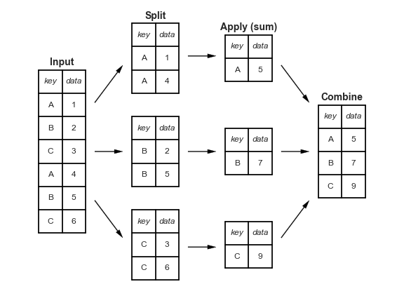
Image credit Jake VanderPlas
Summarizing categorical data
Aggregation (or "summary") methods, such as .sum() and .mean() can be used to calculate their respective statistics on subsets (groups) in the data. When the mean is computed, the default behavior is to ignore NA values, so they only need to be dropped if they are to be excluded from the visual output.
world_data.groupby('region')['population'].sum()
region
Africa       59192998600
Americas     63837885500
Asia        330133218800
Europe       98766930400
Oceania       2422277600
Name: population, dtype: int64
The output here is a series that is indexed with the grouped variable (the region) as the index and the result of the aggregation (the total population) as the values (conceptually, the only column).
These populations numbers are abnormally high because the summary is made for all the years instead of only one. To view only the data from this year, use the learnt methods to subset for only 2018. Compare these results to the picture in the survey that placed 4 million people in Asia and 1 million in each of the other regions.
world_data_2018 = world_data.loc[world_data['year'] == 2018]
world_data_2018.groupby('region')['population'].sum()
region
Africa      1286388200
Americas    1010688000
Asia        4514211000
Europe       742109000
Oceania       40212000
Name: population, dtype: int64
These numbers are closer to the survey we took earlier.
Individual countries can be selected from the resulting series using loc[], just as previously.
avg_density = world_data_2018.groupby('region')['population'].sum()
avg_density.loc[['Asia', 'Europe']]
region
Asia      4514211000
Europe     742109000
Name: population, dtype: int64
As a shortcut, loc[] can be omitted when indexing a series. This is similar to selecting columns from a data frame with just [].
avg_density[['Asia', 'Europe']]
region
Asia      4514211000
Europe     742109000
Name: population, dtype: int64
This indexing can be used to normalize the population numbers to the region of interest.
region_pop_2018 = world_data_2018.groupby('region')['population'].sum()
region_pop_2018 / region_pop_2018['Europe']
region
Africa      1.733422
Americas    1.361913
Asia        6.082949
Europe      1.000000
Oceania     0.054186
Name: population, dtype: float64
There are 6 times as many people living in Asia than in Europe.
Groups can also be created from multiple columns, e.g. it could be interesting to compare the how densely populated countries are on average in different income brackets around the world.
world_data_2018.groupby(['region', 'income_group'])['pop_density'].mean()
region    income_group
Africa    High             207.000000
          Low              118.640741
          Lower middle      69.331250
          Upper middle      94.457500
Americas  High             136.426000
          Low              403.000000
          Lower middle     113.950000
          Upper middle      92.931875
Asia      High            1121.654545
          Low              115.866667
          Lower middle     262.606471
          Upper middle     235.447692
Europe    High             176.563214
          Lower middle      99.500000
          Upper middle      67.832222
Oceania   High              10.610000
          Lower middle      52.500000
          Upper middle      90.266667
Name: pop_density, dtype: float64
Note that income_group is an ordinal variable, i.e. a categorical variable with an inherent order to it. Here, pandas has not listed the values of that variable in the order we would expect (low, lower-middle, upper-middle, high). The order of a variable can be specified in the data frame itself, using the top level pandas function Categorical().
# Reassign in the main data frame since we will use more than just the 2018 data later
world_data['income_group'] = (
    pd.Categorical(world_data['income_group'], ordered=True,
                   categories=['Low', 'Lower middle', 'Upper middle', 'High'])
)

# Need to recreate the 2018 data frame since the categorical was changed in the main frame
world_data_2018 = world_data.loc[world_data['year'] == 2018]
world_data_2018['income_group'].dtype
CategoricalDtype(categories=['Low', 'Lower middle', 'Upper middle', 'High'], ordered=True)
world_data_2018.groupby(['region', 'income_group'])['pop_density'].mean()
region    income_group
Africa    Low              118.640741
          Lower middle      69.331250
          Upper middle      94.457500
          High             207.000000
Americas  Low              403.000000
          Lower middle     113.950000
          Upper middle      92.931875
          High             136.426000
Asia      Low              115.866667
          Lower middle     262.606471
          Upper middle     235.447692
          High            1121.654545
Europe    Lower middle      99.500000
          Upper middle      67.832222
          High             176.563214
Oceania   Lower middle      52.500000
          Upper middle      90.266667
          High              10.610000
Name: pop_density, dtype: float64
Now the values appear in the order we would expect. The value for Asia in the high income bracket looks suspiciously high. It would be interesting to see which countries were averaged to that value.
world_data_2018.loc[(world_data['region'] == 'Asia') &
                    (world_data['income_group'] == 'High'),
                    ['country', 'pop_density']]
| country | pop_density | |
|---|---|---|
| 2627 | Bahrain | 2060.0 |
| 9197 | Cyprus | 129.0 |
| 16862 | Israel | 391.0 |
| 17519 | Japan | 349.0 |
| 18614 | Kuwait | 236.0 |
| 26279 | Oman | 15.6 |
| 28469 | Qatar | 232.0 |
| 29564 | Saudi Arabia | 15.6 |
| 30659 | Singapore | 8270.0 |
| 31973 | South Korea | 526.0 |
| 36791 | United Arab Emirates | 114.0 |
Extreme values, such as the city-state Singapore, can heavily skew averages and it could be a good idea to use a more robust statistics such as the median instead.
world_data_2018.groupby(['region', 'income_group'])['pop_density'].median()
region    income_group
Africa    Low              66.70
          Lower middle     74.75
          Upper middle     12.81
          High            207.00
Americas  Low             403.00
          Lower middle     68.20
          Upper middle     55.95
          High             37.80
Asia      Low              82.35
          Lower middle     92.00
          Upper middle    106.00
          High            236.00
Europe    Lower middle     99.50
          Upper middle     68.70
          High            109.50
Oceania   Lower middle     22.70
          Upper middle     69.90
          High             10.61
Name: pop_density, dtype: float64
The returned series has an index that is a combination of the columns region and sub_region, and referred to as a MultiIndex. The same syntax as previously can be used to select rows on the species-level.
med_density_2018 = world_data_2018.groupby(['region', 'income_group'])['pop_density'].median()
med_density_2018[['Africa', 'Americas']]
region    income_group
Africa    Low              66.70
          Lower middle     74.75
          Upper middle     12.81
          High            207.00
Americas  Low             403.00
          Lower middle     68.20
          Upper middle     55.95
          High             37.80
Name: pop_density, dtype: float64
To select specific values from both levels of the MultiIndex, a list of tuples can be passed to loc[].
med_density_2018.loc[[('Africa', 'High'), ('Americas', 'High')]]
region    income_group
Africa    High            207.0
Americas  High             37.8
Name: pop_density, dtype: float64
To select only the low income values from all region, the xs() (cross section) method can be used.
med_density_2018.xs('Low', level='income_group')
region
Africa       66.70
Americas    403.00
Asia         82.35
Name: pop_density, dtype: float64
The names and values of the index levels can be seen by inspecting the index object.
med_density_2018.index
MultiIndex(levels=[['Africa', 'Americas', 'Asia', 'Europe', 'Oceania'], ['Low', 'Lower middle', 'Upper middle', 'High']],
           labels=[[0, 0, 0, 0, 1, 1, 1, 1, 2, 2, 2, 2, 3, 3, 3, 4, 4, 4], [0, 1, 2, 3, 0, 1, 2, 3, 0, 1, 2, 3, 1, 2, 3, 1, 2, 3]],
           names=['region', 'income_group'])
Although MultiIndexes offer succinct and fast ways to access data, they also requires memorization of additional syntax and are strictly speaking not essential unless speed is of particular concern. It can therefore be easier to reset the index, so that all values are stored in columns.
med_density_2018_res = med_density_2018.reset_index()
med_density_2018_res
| region | income_group | pop_density | |
|---|---|---|---|
| 0 | Africa | Low | 66.70 |
| 1 | Africa | Lower middle | 74.75 |
| 2 | Africa | Upper middle | 12.81 |
| 3 | Africa | High | 207.00 |
| 4 | Americas | Low | 403.00 |
| 5 | Americas | Lower middle | 68.20 |
| 6 | Americas | Upper middle | 55.95 |
| 7 | Americas | High | 37.80 |
| 8 | Asia | Low | 82.35 |
| 9 | Asia | Lower middle | 92.00 |
| 10 | Asia | Upper middle | 106.00 |
| 11 | Asia | High | 236.00 |
| 12 | Europe | Lower middle | 99.50 |
| 13 | Europe | Upper middle | 68.70 |
| 14 | Europe | High | 109.50 |
| 15 | Oceania | Lower middle | 22.70 |
| 16 | Oceania | Upper middle | 69.90 |
| 17 | Oceania | High | 10.61 |
After resetting the index, the same comparison syntax introduced earlier can be used instead of xs() or passing lists of tuples to loc[].
med_density_2018_asia = med_density_2018_res.loc[med_density_2018_res['income_group'] == 'Low']
med_density_2018_asia
| region | income_group | pop_density | |
|---|---|---|---|
| 0 | Africa | Low | 66.70 |
| 4 | Americas | Low | 403.00 |
| 8 | Asia | Low | 82.35 |
reset_index() grants the freedom of not having to work with indexes, but it is still worth keeping in mind that selecting on an index level with xs() can be orders of magnitude faster than using boolean comparisons (on large data frames).
The opposite operation (to create an index) can be performed with set_index() on any column (or combination of columns) that creates an index with unique values.
med_density_2018_asia.set_index(['region', 'income_group'])
| pop_density | ||
|---|---|---|
| region | income_group | |
| Africa | Low | 66.70 |
| Americas | Low | 403.00 |
| Asia | Low | 82.35 |
Challenge
Which is the highest population density in each region?
The low income group for the Americas had the same population density for both the mean and the median. This could mean that there are few observations in this group. List all the low income countries in the Americas.
# Challenge solutions

# 1.
world_data_2018.groupby('region')['pop_density'].max()
region
Africa       625.0
Americas     666.0
Asia        8270.0
Europe      1350.0
Oceania      151.0
Name: pop_density, dtype: float64
# This will be a challenge

# 2.
world_data_2018.loc[(world_data['region'] == 'Americas') & (world_data['income_group'] == 'Low'), ['country', 'pop_density']]
| country | pop_density | |
|---|---|---|
| 14891 | Haiti | 403.0 |
Multiple aggregations on grouped data
Since the same grouped data frame will be used in multiple code chunks below, this can be assigned to a new variable instead of typing out the grouping expression each time.
grouped_world_data = world_data_2018.groupby(['region', 'sub_region'])
grouped_world_data['life_expectancy'].mean()
region    sub_region
Africa    Northern Africa                    74.716667
          Sub-Saharan Africa                 63.682609
Americas  Latin America and the Caribbean    75.600000
          Northern America                   80.650000
Asia      Central Asia                       71.340000
          Eastern Asia                       76.440000
          South-eastern Asia                 73.630000
          Southern Asia                      72.211111
          Western Asia                       76.122222
Europe    Eastern Europe                     75.110000
          Northern Europe                    80.140000
          Southern Europe                    79.466667
          Western Europe                     82.100000
Oceania   Australia and New Zealand          82.350000
          Melanesia                          63.700000
          Micronesia                         62.200000
          Polynesia                          71.550000
Name: life_expectancy, dtype: float64
Instead of using the mean() or sum() methods directly, the more general agg() method could be called to aggregate by any existing aggregation functions. The equivalent to the mean() method would be to call agg() and specify 'mean'.
grouped_world_data['life_expectancy'].agg('mean')
region    sub_region
Africa    Northern Africa                    74.716667
          Sub-Saharan Africa                 63.682609
Americas  Latin America and the Caribbean    75.600000
          Northern America                   80.650000
Asia      Central Asia                       71.340000
          Eastern Asia                       76.440000
          South-eastern Asia                 73.630000
          Southern Asia                      72.211111
          Western Asia                       76.122222
Europe    Eastern Europe                     75.110000
          Northern Europe                    80.140000
          Southern Europe                    79.466667
          Western Europe                     82.100000
Oceania   Australia and New Zealand          82.350000
          Melanesia                          63.700000
          Micronesia                         62.200000
          Polynesia                          71.550000
Name: life_expectancy, dtype: float64
This general approach is more flexible and powerful since multiple aggregation functions can be applied in the same line of code by passing them as a list to agg(). For instance, the standard deviation and mean could be computed in the same call by passing them in a list.
grouped_world_data['life_expectancy'].agg(['mean', 'std'])
| mean | std | ||
|---|---|---|---|
| region | sub_region | ||
| Africa | Northern Africa | 74.716667 | 3.510793 |
| Sub-Saharan Africa | 63.682609 | 4.540108 | |
| Americas | Latin America and the Caribbean | 75.600000 | 3.721559 |
| Northern America | 80.650000 | 2.192031 | |
| Asia | Central Asia | 71.340000 | 0.808084 |
| Eastern Asia | 76.440000 | 6.566430 | |
| South-eastern Asia | 73.630000 | 4.835298 | |
| Southern Asia | 72.211111 | 6.426983 | |
| Western Asia | 76.122222 | 4.585214 | |
| Europe | Eastern Europe | 75.110000 | 2.711478 |
| Northern Europe | 80.140000 | 2.958678 | |
| Southern Europe | 79.466667 | 2.694889 | |
| Western Europe | 82.100000 | 0.804156 | |
| Oceania | Australia and New Zealand | 82.350000 | 0.777817 |
| Melanesia | 63.700000 | 1.961292 | |
| Micronesia | 62.200000 | NaN | |
| Polynesia | 71.550000 | 1.202082 |
The returned output is in this case a data frame and the MultiIndex is indicated in bold font.
By passing a dictionary to .agg() it is possible to apply different aggregations to the different columns. Long code statements can be broken down into multiple lines if they are enclosed by parentheses, brackets or braces, something that will be described in detail later.
grouped_world_data[['population', 'income']].agg(
    {'population': 'sum',
     'income': ['min', 'median', 'max']
    }
)
| population | income | ||||
|---|---|---|---|---|---|
| sum | min | median | max | ||
| region | sub_region | ||||
| Africa | Northern Africa | 237270000 | 4440 | 11200 | 18300 |
| Sub-Saharan Africa | 1049118200 | 629 | 1985 | 27500 | |
| Americas | Latin America and the Caribbean | 646688000 | 1710 | 13700 | 30300 |
| Northern America | 364000000 | 43800 | 49350 | 54900 | |
| Asia | Central Asia | 71890000 | 2920 | 6690 | 24200 |
| Eastern Asia | 1626920000 | 1390 | 16000 | 39100 | |
| South-eastern Asia | 655870000 | 1490 | 7255 | 83900 | |
| Southern Asia | 1887261000 | 1870 | 6890 | 17400 | |
| Western Asia | 272270000 | 2430 | 20750 | 121000 | |
| Europe | Eastern Europe | 291970000 | 5330 | 24100 | 32300 |
| Northern Europe | 104478000 | 25500 | 43450 | 65600 | |
| Southern Europe | 151681000 | 12100 | 24050 | 37900 | |
| Western Europe | 193980000 | 39000 | 45200 | 99000 | |
| Oceania | Australia and New Zealand | 29550000 | 36400 | 41100 | 45800 |
| Melanesia | 10237000 | 2110 | 2850 | 9420 | |
| Micronesia | 118000 | 1890 | 1890 | 1890 | |
| Polynesia | 307000 | 5500 | 5725 | 5950 | |
There are plenty of aggregation methods available in pandas (e.g. sem, mad, sum, most of which can be seen at the end of this section in the pandas documentation, or explored using tab-complete on the grouped data frame).
# This is a side note, no need to bring up unless someone has issues
# Tab completion might only work like this:
# find_agg_methods = grouped_world_data['weight']
# find_agg_methods.<tab>
Even if a function is not part of the pandas library, it can be passed to agg().
import numpy as np

grouped_world_data['pop_density'].agg(np.mean)
region    sub_region
Africa    Northern Africa                     50.113333
          Sub-Saharan Africa                 108.143043
Americas  Latin America and the Caribbean    126.558966
          Northern America                    19.880000
Asia      Central Asia                        38.504000
          Eastern Asia                       248.202000
          South-eastern Asia                 961.110000
          Southern Asia                      460.388889
          Western Asia                       298.355556
Europe    Eastern Europe                      88.629000
          Northern Europe                     64.897000
          Southern Europe                    202.166667
          Western Europe                     256.000000
Oceania   Australia and New Zealand           10.610000
          Melanesia                           28.475000
          Micronesia                         146.000000
          Polynesia                          110.450000
Name: pop_density, dtype: float64
Any function can be passed like this, including user-created functions.
Challenge
What's the mean life expectancy for each income group in 2018?
What's the min, median, and max life expectancies for each income group within each region?
# Challenge solutions

# 1.
world_data_2018.groupby('income_group')['life_expectancy'].mean()
income_group
Low             63.744118
Lower middle    69.053488
Upper middle    74.283673
High            79.919231
Name: life_expectancy, dtype: float64
# 2.
world_data_2018.groupby(['region', 'income_group'])['life_expectancy'].agg(['min', 'median', 'max'])
| min | median | max | ||
|---|---|---|---|---|
| region | income_group | |||
| Africa | Low | 51.6 | 62.50 | 68.3 |
| Lower middle | 51.1 | 66.35 | 78.0 | |
| Upper middle | 63.5 | 67.10 | 77.9 | |
| High | 74.2 | 74.20 | 74.2 | |
| Americas | Low | 64.5 | 64.50 | 64.5 |
| Lower middle | 73.1 | 74.90 | 78.7 | |
| Upper middle | 68.2 | 75.80 | 81.4 | |
| High | 73.4 | 77.60 | 82.2 | |
| Asia | Low | 58.7 | 70.45 | 72.2 |
| Lower middle | 67.9 | 71.50 | 77.8 | |
| Upper middle | 68.0 | 76.50 | 80.5 | |
| High | 76.9 | 80.70 | 84.2 | |
| Europe | Lower middle | 72.3 | 72.35 | 72.4 |
| Upper middle | 71.1 | 75.50 | 78.0 | |
| High | 75.1 | 81.30 | 83.5 | |
| Oceania | Lower middle | 61.1 | 62.90 | 64.3 |
| Upper middle | 65.8 | 70.70 | 72.4 | |
| High | 81.8 | 82.35 | 82.9 |
Additional sections (time permitting)
Using size() to summarize categorical data
When working with data, it is common to want to know the number of observations present for each categorical variable. For this, pandas provides the size() method. For example, to find the number of observations (in this case unique countries during year 2018) per region:
world_data_2018.groupby('region').size()
region
Africa      52
Americas    31
Asia        47
Europe      39
Oceania      9
dtype: int64
size() can also be used when grouping on multiple variables.
world_data_2018.groupby(['region', 'income_group']).size()
region    income_group
Africa    Low             27
          Lower middle    16
          Upper middle     8
          High             1
Americas  Low              1
          Lower middle     4
          Upper middle    16
          High            10
Asia      Low              6
          Lower middle    17
          Upper middle    13
          High            11
Europe    Lower middle     2
          Upper middle     9
          High            28
Oceania   Lower middle     4
          Upper middle     3
          High             2
dtype: int64
If there are many groups, size() is not that useful on its own. For example, it is difficult to quickly find the five most abundant species among the observations.
world_data_2018.groupby('sub_region').size()
sub_region
Australia and New Zealand           2
Central Asia                        5
Eastern Asia                        5
Eastern Europe                     10
Latin America and the Caribbean    29
Melanesia                           4
Micronesia                          1
Northern Africa                     6
Northern America                    2
Northern Europe                    10
Polynesia                           2
South-eastern Asia                 10
Southern Asia                       9
Southern Europe                    12
Sub-Saharan Africa                 46
Western Asia                       18
Western Europe                      7
dtype: int64
Since there are many rows in this output, it would be beneficial to sort the table values and display the most abundant species first. This is easy to do with the sort_values() method.
world_data_2018.groupby('sub_region').size().sort_values()
sub_region
Micronesia                          1
Australia and New Zealand           2
Polynesia                           2
Northern America                    2
Melanesia                           4
Eastern Asia                        5
Central Asia                        5
Northern Africa                     6
Western Europe                      7
Southern Asia                       9
Northern Europe                    10
South-eastern Asia                 10
Eastern Europe                     10
Southern Europe                    12
Western Asia                       18
Latin America and the Caribbean    29
Sub-Saharan Africa                 46
dtype: int64
That's better, but it could be helpful to display the most abundant species on top. In other words, the output should be arranged in descending order.
world_data_2018.groupby('sub_region').size().sort_values(ascending=False).head(5)
sub_region
Sub-Saharan Africa                 46
Latin America and the Caribbean    29
Western Asia                       18
Southern Europe                    12
Eastern Europe                     10
dtype: int64
Looks good! By now, the code statement has grown quite long because many methods have been chained together. It can be tricky to keep track of what is going on in long method chains. To make the code more readable, it can be broken up multiple lines by adding a surrounding parenthesis.
(world_data_2018
     .groupby('sub_region')
     .size()
     .sort_values(ascending=False)
     .head(5)
)
sub_region
Sub-Saharan Africa                 46
Latin America and the Caribbean    29
Western Asia                       18
Southern Europe                    12
Eastern Europe                     10
dtype: int64
This looks neater and makes long method chains easier to reads. There is no absolute rule for when to break code into multiple line, but always try to write code that is easy for collaborators (your most common collaborator is a future version of yourself!) to understand.
pandas actually has a convenience function for returning the top five results, so the values don't need to be sorted explicitly.
(world_data_2018
     .groupby(['sub_region'])
     .size()
     .nlargest() # the default is 5
)
sub_region
Sub-Saharan Africa                 46
Latin America and the Caribbean    29
Western Asia                       18
Southern Europe                    12
Eastern Europe                     10
dtype: int64
To include more attributes about these countries, add those columns to groupby().
(world_data_2018
     .groupby(['region', 'sub_region'])
     .size()
     .nlargest() # the default is 5
)
region    sub_region
Africa    Sub-Saharan Africa                 46
Americas  Latin America and the Caribbean    29
Asia      Western Asia                       18
Europe    Southern Europe                    12
Asia      South-eastern Asia                 10
dtype: int64
world_data.head()
| country | year | population | region | sub_region | income_group | life_expectancy | income | children_per_woman | child_mortality | pop_density | co2_per_capita | years_in_school_men | years_in_school_women | population_income | |
|---|---|---|---|---|---|---|---|---|---|---|---|---|---|---|---|
| 0 | Afghanistan | 1800 | 3280000 | Asia | Southern Asia | Low | 28.2 | 603 | 7.0 | 469.0 | NaN | NaN | NaN | NaN | 1977840000 |
| 1 | Afghanistan | 1801 | 3280000 | Asia | Southern Asia | Low | 28.2 | 603 | 7.0 | 469.0 | NaN | NaN | NaN | NaN | 1977840000 |
| 2 | Afghanistan | 1802 | 3280000 | Asia | Southern Asia | Low | 28.2 | 603 | 7.0 | 469.0 | NaN | NaN | NaN | NaN | 1977840000 |
| 3 | Afghanistan | 1803 | 3280000 | Asia | Southern Asia | Low | 28.2 | 603 | 7.0 | 469.0 | NaN | NaN | NaN | NaN | 1977840000 |
| 4 | Afghanistan | 1804 | 3280000 | Asia | Southern Asia | Low | 28.2 | 603 | 7.0 | 469.0 | NaN | NaN | NaN | NaN | 1977840000 |
Challenge
- How many countries are there in each income group worldwide?
- Assign the variable name
world_data_2015to a data frame containing only the values from year 2015 (e.g. the same way asworld_data_2018was created)
- For those countries where women went to school longer than men, how many are in each income group.
- Do the same as above but for countries where men went to school longer than women. What does this distribution tell you?
# Challenge solutions
# 1.
world_data_2018.groupby('income_group').size()
income_group
Low             34
Lower middle    43
Upper middle    49
High            52
dtype: int64
# 2
world_data_2015 = world_data.loc[world_data['year'] == 2015]
# 3a
world_data_2015.loc[world_data_2015['years_in_school_men'] < world_data_2015['years_in_school_women']].groupby('income_group').size()
income_group
Low              0
Lower middle    14
Upper middle    33
High            47
dtype: int64
# 3b
world_data_2015.loc[world_data_2015['years_in_school_men'] > world_data_2015['years_in_school_women']].groupby('income_group').size()
income_group
Low             34
Lower middle    29
Upper middle    11
High             5
dtype: int64
Data cleaning tips
dropna() removes both explicit NaN values and value that pandas are assumed to be NaN, such as the non-numeric values in the life_expectancy column. Non-numeric values can also be coerced into explicit NaN values via the to_numeric() top level function.
pd.to_numeric(clean_df['life_expectancy'], errors='coerce')
0     71.5
1      NaN
2     71.6
3      NaN
4     71.7
5     72.0
6     70.0
7     70.0
8     70.1
9     70.2
10     NaN
11    70.4
Name: life_expectancy, dtype: float64