
python-awips: Working with Upper Air Obs
Unidata AMS 2021 Student Conference
Focuses
- Retreive upper air vertical profile data from EDEX server.
- Use EDEX to get the pressure, temperature, dewpoint lines and wind profile data for the Upper Air observation.
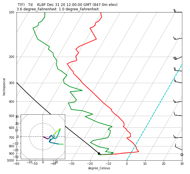
- Plot a Skew-T/Log-P plot with Hodograph using Matplotlib and Metpy.
Objectives
Imports
In [ ]:
from awips.dataaccess import DataAccessLayer
import matplotlib.tri as mtri
import matplotlib.pyplot as plt
from mpl_toolkits.axes_grid1.inset_locator import inset_axes
import numpy as np
import math
from metpy.calc import wind_speed, wind_components, lcl, dry_lapse, parcel_profile
from metpy.plots import SkewT, Hodograph
from metpy.units import units, concatenate
1. Define Data Request
If you read through the python-awips: How to Access Data training, you will know that we need to set an EDEX url to access our server, and then we create a data request. In this example we use bufrua as the data type to define our request. We also set some parameters and the location name. The bufrua plugin returns separate objects for parameters at mandatory levels and at significant temperature levels. For the Skew-T/Log-P plot, significant temperature levels are used to plot the pressure, temperature, and dewpoint lines, while mandatory levels are used to plot the wind profile.
In [ ]:
# Create an EDEX data request
DataAccessLayer.changeEDEXHost("edex-cloud.unidata.ucar.edu")
request = DataAccessLayer.newDataRequest()
request.setDatatype("bufrua")

# set parameters, including the mandatory and significant parameters
MAN_PARAMS = set(['prMan', 'htMan', 'tpMan', 'tdMan', 'wdMan', 'wsMan'])
SIGT_PARAMS = set(['prSigT', 'tpSigT', 'tdSigT'])
request.setParameters("wmoStaNum", "validTime", "rptType", "staElev", "numMand",
                      "numSigT", "numSigW", "numTrop", "numMwnd", "staName")
request.getParameters().extend(MAN_PARAMS)
request.getParameters().extend(SIGT_PARAMS)

# Set station ID (not name)
request.setLocationNames("72562") #KLBF

# Take a look at our request
print(request)
In [ ]:
# Get all times
datatimes = DataAccessLayer.getAvailableTimes(request)

# Get most recent record
response = DataAccessLayer.getGeometryData(request,times=datatimes[-1].validPeriod)
In [ ]:
# Initialize data arrays
tdMan,tpMan,prMan,wdMan,wsMan = np.array([]),np.array([]),np.array([]),np.array([]),np.array([])
prSig,tpSig,tdSig = np.array([]),np.array([]),np.array([])
manGeos = []
sigtGeos = []

# Build  arrays
for ob in response:
    parm_array = ob.getParameters()
    if set(parm_array) & MAN_PARAMS:
        manGeos.append(ob)
        prMan = np.append(prMan,ob.getNumber("prMan"))
        tpMan, tpUnit = np.append(tpMan,ob.getNumber("tpMan")), ob.getUnit("tpMan")
        tdMan, tdUnit = np.append(tdMan,ob.getNumber("tdMan")), ob.getUnit("tdMan")
        wdMan = np.append(wdMan,ob.getNumber("wdMan"))
        wsMan, wsUnit = np.append(wsMan,ob.getNumber("wsMan")), ob.getUnit("wsMan")
        continue
    if set(parm_array) & SIGT_PARAMS:
        sigtGeos.append(ob)
        prSig = np.append(prSig,ob.getNumber("prSigT"))
        tpSig = np.append(tpSig,ob.getNumber("tpSigT"))
        tdSig = np.append(tdSig,ob.getNumber("tdSigT"))
        continue
In [ ]:
# Sort mandatory levels (but not sigT levels) because of the 1000.MB interpolation inclusion
ps = prMan.argsort()[::-1]
wpres = prMan[ps]
direc = wdMan[ps]
spd   = wsMan[ps]
tman = tpMan[ps]
dman = tdMan[ps]

# Flag missing data
prSig[prSig <= -9999] = np.nan
tpSig[tpSig <= -9999] = np.nan
tdSig[tdSig <= -9999] = np.nan
wpres[wpres <= -9999] = np.nan
tman[tman <= -9999] = np.nan
dman[dman <= -9999] = np.nan
direc[direc <= -9999] = np.nan
spd[spd <= -9999] = np.nan

# assign units
p = (prSig/100) * units.mbar
wpres = (wpres/100) * units.mbar
u,v = wind_components(spd * units.knots, np.deg2rad(direc))

if tpUnit == 'K':
    T = (tpSig-273.15) * units.degC
    Td = (tdSig-273.15) * units.degC
    tman = tman * units.degC
    dman = dman * units.degC
In [ ]:
# Create SkewT/LogP
plt.rcParams['figure.figsize'] = (10, 12)
skew = SkewT()
skew.plot(p, T, 'r', linewidth=2)
skew.plot(p, Td, 'g', linewidth=2)
skew.plot_barbs(wpres, u, v)
skew.ax.set_ylim(1000, 100)
skew.ax.set_xlim(-60, 30)

title_string = " T(F)   Td   "
title_string +=  " " + str(ob.getString("staName"))
title_string += " " + str(ob.getDataTime().getRefTime())
title_string += " (" + str(ob.getNumber("staElev")) + "m elev)"
title_string += "\n" + str(round(T[0].to('degF').item(),1))
title_string += "  " + str(round(Td[0].to('degF').item(),1))
plt.title(title_string, loc='left')

# Calculate LCL height and plot as black dot
lcl_pressure, lcl_temperature = lcl(p[0], T[0], Td[0])
skew.plot(lcl_pressure, lcl_temperature, 'ko', markerfacecolor='black')

# Calculate full parcel profile and add to plot as black line
prof = parcel_profile(p, T[0], Td[0]).to('degC')
skew.plot(p, prof, 'k', linewidth=2)

# An example of a slanted line at constant T -- in this case the 0 isotherm
l = skew.ax.axvline(0, color='c', linestyle='--', linewidth=2)

# Draw hodograph
ax_hod = inset_axes(skew.ax, '30%', '30%', loc=3)
h = Hodograph(ax_hod, component_range=max(wsMan))
h.add_grid(increment=20)
h.plot_colormapped(u, v, spd)

# Show the plot
plt.show()
See also
Documentation for:
- awips.DataAccessLayer
- awips.PyGeometryData
- matplotlib.pyplot
- metpy.plots.SkewT
- metpy.plots.Hodograph