
python-awips: Working with Satellite Data
Unidata AMS 2021 Student Conference
Focuses
- Investigate what satellite data is available from an EDEX server.
- Define map properties in a function that can be used to plot multiple images.
- Retreive Mesoscale GOES satellite grid data from an EDEX server.
- Use matplotlib pcolormesh to plot the colorized images with a colorbar.
Objectives
- Define Data Request
- View Optional Identifiers
- View Sources
- View Creating Entities
- View Sector IDs
- Create a Satellite Product Tree
- Define Map Properties
- Plot Image Data!
Imports
from awips.dataaccess import DataAccessLayer
import cartopy.crs as ccrs
import cartopy.feature as cfeat
import matplotlib.pyplot as plt
from cartopy.mpl.gridliner import LONGITUDE_FORMATTER, LATITUDE_FORMATTER
import numpy as np
import datetime
1. Define Data Request
If you read through the python-awips: How to Access Data training, you will know that we need to set an EDEX url to access our server, and then we create a data request. In this example we use satellite as the data type to define our request.
# Create an EDEX data request
DataAccessLayer.changeEDEXHost("edex-cloud.unidata.ucar.edu")
request = DataAccessLayer.newDataRequest()
request.setDatatype("satellite")

# Take a look at our request
print(request)
# get optional identifiers for satellite datatype
identifiers = set(DataAccessLayer.getOptionalIdentifiers(request))

print("Available Identifiers:")
for id in identifiers:
    if id.lower() == 'datauri':
        continue
    print(" - " + id)
# Show available sources
identifier = "source"
sources = DataAccessLayer.getIdentifierValues(request, identifier)
print(identifier + ":")
print(list(sources))
# Show available creatingEntities
identifier = "creatingEntity"
creatingEntities = DataAccessLayer.getIdentifierValues(request, identifier)
print(identifier + ":")
print(list(creatingEntities))
# Show available sectorIDs
identifier = "sectorID"
sectorIDs = DataAccessLayer.getIdentifierValues(request, identifier)
print(identifier + ":")
print(list(sectorIDs))
6. Create a Satellite Product Tree
By cycling through all the identifiers, a detailed overview of all available products can be created. In this example, first creatingEntity is used, and then availableLocationNames, and availableParameters are used to build the product list further.
Note: The identifieres source and sectorID are not used in this tree, but this is only one way to construct such a product overview.
# Construct a full satellite product tree
for entity in creatingEntities:
    print(entity)
    # Create a new request each time through so only one Identifer is set per request
    request = DataAccessLayer.newDataRequest("satellite")
    request.addIdentifier("creatingEntity", entity)
    # Group by available locations
    availableSectors = DataAccessLayer.getAvailableLocationNames(request)
    availableSectors.sort()
    for sector in availableSectors:
        print(" - " + sector)
        request.setLocationNames(sector)
        # Get all available products
        availableProducts = DataAccessLayer.getAvailableParameters(request)
        availableProducts.sort()
        for product in availableProducts:
            print("    - " + product)
7. Define Map Properties
In order to plot more than one image, it's easiest to define common logic in a function. Here, a new function called make_map is defined. This function uses the matplotlib.pyplot package (plt) to create a figure and axis. The coastlines (continental boundaries) are added, along with lat/lon grids.
def make_map(bbox, projection=ccrs.PlateCarree()):
    fig, ax = plt.subplots(figsize=(10,12),
            subplot_kw=dict(projection=projection))
    if bbox[0] is not np.nan:
        ax.set_extent(bbox)
    ax.coastlines(resolution='50m')
    gl = ax.gridlines(draw_labels=True)
    gl.top_labels = gl.right_labels = False
    gl.xformatter = LONGITUDE_FORMATTER
    gl.yformatter = LATITUDE_FORMATTER
    return fig, ax
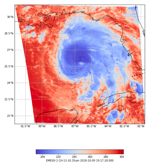
8. Plot Image Data!
For this example, use Channel 13 on the two mesoscale sectors from GOES-East satellite. Create a figure to contain the plot. Create a new Data Request for each sector and set the location and parameters on it. Limit the data to the most recently acquired image using the getAvailableTimes function. Then use pcolormesh to create a plot from the data in the response in the GridData object.
Note: You may see a warning appear with a red background, this is okay, and will go away with subsequent runs of the cell.
# Specify the sectors - GOES East Mesocales
sectors = ["EMESO-1","EMESO-2"]
# Create a figure to contain all subplots
fig = plt.figure(figsize=(16,7*len(sectors)))

# Cycle through the sectors to create and plot recent data from each one
for i, sector in enumerate(sectors):

    # Create the Ch 13 data request
    request = DataAccessLayer.newDataRequest()
    request.setDatatype("satellite")
    request.setLocationNames(sector)
    request.setParameters("CH-13-10.35um")

    # Get the available times
    utc = datetime.datetime.utcnow()
    times = DataAccessLayer.getAvailableTimes(request)

    # Get the grid data using the latest time
    response = DataAccessLayer.getGridData(request, [times[-1]])
    grid = response[0]
    data = grid.getRawData()
    lons,lats = grid.getLatLonCoords()

    # Create the bounding box from the grid data
    bbox = [lons.min(), lons.max(), lats.min(), lats.max()]

    # Draw a new subplot based on the bounding box
    fig, ax = make_map(bbox=bbox)

    # Add state boundaries where available
    states = cfeat.NaturalEarthFeature(category='cultural', name='admin_1_states_provinces_lines', scale='50m', facecolor='none')
    ax.add_feature(states, linestyle=':')

    # Create the color scale
    cs = ax.pcolormesh(lons, lats, data, cmap='coolwarm')

    #Create the colorbar and add a label
    cbar = fig.colorbar(cs, shrink=0.6, orientation='horizontal')
    cbar.set_label(sector + " " + grid.getParameter() + " " \
    + str(grid.getDataTime().getRefTime()))
See also
Documentation for:
- awips.DataAccessLayer
- awips.PyGridData
- matplotlib.pyplot
- matplotlib.pyplot.pcolormesh
- matplotlib.pyplot.subplot