
python-awips: Working with the Maps and Topo Databases
Unidata AMS 2021 Student Conference
Focuses
- Use the AWIPS Maps Database to access GIS objects which are returned as Shapely geometries (Polygon, Point, MultiLineString, etc.) and can be easily plotted by Matplotlib, Cartopy, MetPy, and other packages.
- Use maps and topo data types to obtain GIS data from the AWIPS databases.
- Note the geometry definition of
the_geomfor each data type, which can be Point, MultiPolygon, or MultiLineString. - Step through how to plot several layers of data onto an image, including: county and state boundaries, CWA boundaries, interstates, cities, lakes, rivers, and topograpy.
Objectives
- Define Map Data Request
- Define Map Properties
- Draw County and State Boundaries
- Draw CWA Boundary
- Draw Interstates
- Draw Nearby Cities
- Draw Lakes
- Draw Major Rivers
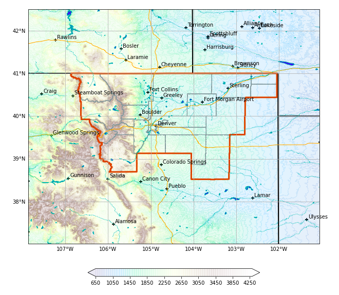
- Draw Topography
Imports
from __future__ import print_function
from awips.dataaccess import DataAccessLayer
import matplotlib.pyplot as plt
import cartopy.crs as ccrs
import numpy as np
from cartopy.mpl.gridliner import LONGITUDE_FORMATTER, LATITUDE_FORMATTER
from cartopy.feature import ShapelyFeature,NaturalEarthFeature
from shapely.geometry import Polygon
from shapely.ops import cascaded_union
import numpy.ma as ma
1. Define the Map Data Request
If you read through the python-awips: How to Access Data training, you will know that we need to set an EDEX url to access our server, and then we create a data request. In this example we use maps as the data type to define our request. We'll use Boulder as our location, so set the Location Name on the request to BDU. Then add several Identifiers for various fields of interest.
# Create EDEX data request
DataAccessLayer.changeEDEXHost("edex-cloud.unidata.ucar.edu")
request = DataAccessLayer.newDataRequest('maps')
request.addIdentifier('table', 'mapdata.county')

# Define a WFO ID for location
# tie this ID to the mapdata.county column "cwa" for filtering
request.setLocationNames('BOU')
request.addIdentifier('cwa', 'BOU')

# enable location filtering (inLocation)
# locationField is tied to the above cwa definition (BOU)
request.addIdentifier('geomField', 'the_geom')
request.addIdentifier('inLocation', 'true')
request.addIdentifier('locationField', 'cwa')

# take a look at the request
print(request)
2. Define Map Properties
If more than one plot is drawn, then it's easiest to define common logic in a function. Here, a new function called make_map is defined. This function uses the matplotlib.pyplot package (plt) to create a figure and axis. The coastlines (continental boundaries) are added, along with lat/lon grids.
Note: We only use this function once in this notebook, but it's in here as an example of how to write a function and use it, for future reference.
# Standard map plot
def make_map(bbox, projection=ccrs.PlateCarree()):
    fig, ax = plt.subplots(figsize=(12,12),
            subplot_kw=dict(projection=projection))
    ax.set_extent(bbox)
    ax.coastlines(resolution='50m')
    gl = ax.gridlines(draw_labels=True)
    gl.top_labels = gl.right_labels = False
    gl.xformatter = LONGITUDE_FORMATTER
    gl.yformatter = LATITUDE_FORMATTER
    return fig, ax
3. Draw County and State Boundaries
Start by getting the GeometryData back from EDEX for the map request. We'll create a plot of the county boundaries for the WFO (in this case Boulder - BDU). Add in the
# Get response and create dict of county geometries
response = DataAccessLayer.getGeometryData(request, [])

# Populate an array of the counties for BDU
counties = np.array([])
for ob in response:
    counties = np.append(counties,ob.getGeometry())


# All WFO counties merged to a single Polygon
merged_counties = cascaded_union(counties)
envelope = merged_counties.buffer(2)
boundaries=[merged_counties]

# Get bounds of this merged Polygon to use as buffered map extent
bounds = merged_counties.bounds
bbox=[bounds[0]-1,bounds[2]+1,bounds[1]-1.5,bounds[3]+1.5]

# Create the map using our defined function
fig, ax = make_map(bbox=bbox)

# Plot state boundaries handled by Cartopy
states = NaturalEarthFeature(category='cultural', name='admin_1_states_provinces_lines', scale='50m', facecolor='none')
ax.add_feature(states, linestyle='-', edgecolor='black',linewidth=2)

# Plot CWA counties
for i, geom in enumerate(counties):
    cbounds = Polygon(geom)
    intersection = cbounds.intersection
    geoms = (intersection(geom) for geom in counties if cbounds.intersects(geom))
    shape_feature = ShapelyFeature(geoms,ccrs.PlateCarree(), facecolor='none', linestyle="-",edgecolor='#86989B')
    ax.add_feature(shape_feature)
# use the merged polygon to draw the CWA boundary
geom = boundaries[0]
gbounds = Polygon(geom)
intersection = gbounds.intersection
geoms = (intersection(geom) for geom in boundaries if gbounds.intersects(geom))
shape_feature = ShapelyFeature(geoms,ccrs.PlateCarree(), facecolor='none', linestyle="-",linewidth=3.,edgecolor='#cc5000')
ax.add_feature(shape_feature)

# Display the plot
fig
# Create new request to get interstate polygons from the EDEX server
request = DataAccessLayer.newDataRequest('maps', envelope=envelope)
request.addIdentifier('table', 'mapdata.interstate')
request.addIdentifier('geomField', 'the_geom')
request.setParameters('name')
interstates = DataAccessLayer.getGeometryData(request, [])

# Plot interstates
for ob in interstates:
    shape_feature = ShapelyFeature(ob.getGeometry(),ccrs.PlateCarree(), facecolor='none', linestyle="-",edgecolor='orange')
    ax.add_feature(shape_feature)

# Display the plot
fig
# Create new request for local cities
request = DataAccessLayer.newDataRequest('maps', envelope=envelope)
request.addIdentifier('table', 'mapdata.city')
request.addIdentifier('geomField', 'the_geom')
request.setParameters('name','population','prog_disc')
cities = DataAccessLayer.getGeometryData(request, [])

citylist = []
cityname = []
# For BOU, progressive disclosure values above 50 and pop above 5000 looks good
for ob in cities:
    if ob.getString("population"):
        if ob.getNumber("prog_disc") > 50:
            if int(ob.getString("population")) > 5000:
                citylist.append(ob.getGeometry())
                cityname.append(ob.getString("name"))

# Plot city markers
ax.scatter([point.x for point in citylist], [point.y for point in citylist], transform=ccrs.PlateCarree(),marker="+",facecolor='black')
# Plot city names
for i, txt in enumerate(cityname):
    ax.annotate(txt, (citylist[i].x,citylist[i].y), xytext=(3,3), textcoords="offset points")

# Display the plot
fig
# Create a request for lakes
request = DataAccessLayer.newDataRequest('maps', envelope=envelope)
request.addIdentifier('table', 'mapdata.lake')
request.addIdentifier('geomField', 'the_geom')
request.setParameters('name')

# Get lake geometries
response = DataAccessLayer.getGeometryData(request, [])
lakes = np.array([])
for ob in response:
    lakes = np.append(lakes,ob.getGeometry())

# Plot lakes
for i, geom in enumerate(lakes):
    cbounds = Polygon(geom)
    intersection = cbounds.intersection
    geoms = (intersection(geom) for geom in lakes if cbounds.intersects(geom))
    shape_feature = ShapelyFeature(geoms,ccrs.PlateCarree(), facecolor='blue', linestyle="-",edgecolor='#20B2AA')
    ax.add_feature(shape_feature)

# Display the plot
fig
# Create a new request for major rivers
request = DataAccessLayer.newDataRequest('maps', envelope=envelope)
request.addIdentifier('table', 'mapdata.majorrivers')
request.addIdentifier('geomField', 'the_geom')
request.setParameters('pname')
rivers = DataAccessLayer.getGeometryData(request, [])

# Plot rivers
for ob in rivers:
    shape_feature = ShapelyFeature(ob.getGeometry(),ccrs.PlateCarree(), facecolor='none', linestyle=":", edgecolor='#20B2AA')
    ax.add_feature(shape_feature)

# Display the plot
fig
# Create new request for l
request = DataAccessLayer.newDataRequest("topo")
request.addIdentifier("group", "/")
request.addIdentifier("dataset", "full")
request.setEnvelope(envelope)
gridData = DataAccessLayer.getGridData(request)
grid=gridData[0]
topo=ma.masked_invalid(grid.getRawData())
lons, lats = grid.getLatLonCoords()
# print(topo.min()) # minimum elevation in our domain (meters)
# print(topo.max()) # maximum elevation in our domain (meters)

# Plot topography
cs = ax.contourf(lons, lats, topo, 80, cmap=plt.get_cmap('terrain'),alpha=0.1, extend='both')
cbar = fig.colorbar(cs, shrink=0.5, orientation='horizontal')
cbar.set_label("topography height in meters")

# Display the plot
fig
See also
Documentation for:
- AWIPS Maps Database Reference List
- awips.DataAccessLayer
- awips.PyGeometryData
- matplotlib.pyplot
- matplotlib.pyplot.subplot
- matplotlib.pyplot.contourf