
Matplotlib: Intermediate
Unidata AMS 2021 Student Conference
Focuses
- Draw multiple plots in the same figure.
- Colorize individual scatter plot points based on some criteria.
- Use imshow, contour and contourf to draw a heat maps and contour plots.
Objectives
- Create Test Data
- Multiple Plots on One Figure
- Colorizing Scatter Plots
- Plot a Heat Map with Imshow
- Plot with Contour
- Plot with Contourf
- Combine Imshow and Contour
Imports
%matplotlib inline
import matplotlib.pyplot as plt
import numpy as np
1. Create Test Data
First, instantiate some test data to work with in this notebook.
# Create the test data to work with
times = np.array([ 93.,  96.,  99., 102., 105., 108., 111., 114., 117.,
                  120., 123., 126., 129., 132., 135., 138., 141., 144.,
                  147., 150., 153., 156., 159., 162.])
temps = np.array([310.7, 308.0, 296.4, 289.5, 288.5, 287.1, 301.1, 308.3,
                  311.5, 305.1, 295.6, 292.4, 290.4, 289.1, 299.4, 307.9,
                  316.6, 293.9, 291.2, 289.8, 287.1, 285.8, 303.3, 310.])
temps_1000 = np.array([316.0, 316.3, 308.9, 304.0, 302.0, 300.8, 306.2, 309.8,
                       313.5, 313.3, 308.3, 304.9, 301.0, 299.2, 302.6, 309.0,
                       311.8, 304.7, 304.6, 301.8, 300.6, 299.9, 306.3, 311.3])
# Fake dewpoint data to plot
dewpoint = 0.9 * temps
dewpoint_1000 = 0.9 * temps_1000
2. Multiple Plots on One Figure
The Matplotlib: Basics notebook explained how to create a figure and add a plot to that figure. It is also possible to add multiple plots to the same figure. In this step, a figure is first created and then multiple plots are added, each with their own titles, axes, etc. Each plot is added using the add_subplot() function, which lays out multiple plots in a grid by passing the number of rows, columns, and which plot within the grid (starting with 1, not 0).
So for example, if you wanted to create a plot in the lower left corner of a (hypothetical) grid of plots with 2 rows and 3 columns, you could write fig.add_subplot(2, 3, 4), where 4 means the 4th plot, counting across rows and down columns."
# Cell content replaced by load magic replacement.
fig = plt.figure(figsize=(10, 6))
ax = fig.add_subplot(1, 2, 1)

# Specify how our lines should look
ax.plot(times, temps, color='tab:red', label='Temperature (surface)')
ax.plot(times, temps_1000, color='tab:red', linestyle=':',
        label='Temperature (isobaric level)')

# Add labels, title, and display settings
ax.set_xlabel('Time')
ax.set_ylabel('Temperature')
ax.set_title('Temperature Forecast')
ax.grid(True)
ax.legend(loc='upper left')

# Create the second plot
ax2 = fig.add_subplot(1, 2, 2, sharex=ax, sharey=ax)
ax2.plot(times, dewpoint, color='tab:green', label='Dewpoint (surface)')
ax2.plot(times, dewpoint_1000, color='tab:green', linestyle=':', marker='o',
         label='Dewpoint (isobaric level)')

# Add labels, title, and display settings
ax2.set_xlabel('Time')
ax2.set_ylabel('Dewpoint')
ax2.set_title('Dewpoint Forecast')
ax2.grid(True)
ax2.legend(loc='upper left')
ax2.set_ylim(257, 312)
ax2.set_xlim(95, 162)
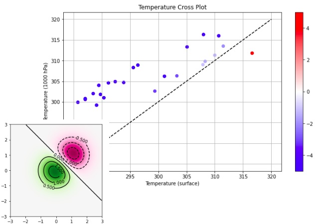
3. Colorizing Scatter Plots
Previously, in the Matplotlib: Basics notebook, an example for drawing scatter plots was provided by setting the linestyle to none, and adding 'o' markers. Another alternative is to use the scatter methods, while these are slower, they allow more visualization options of the data, such as style or color of the individual markers. In this case, the data points will be colorized individually based upon a third variable.
# Create the plot
fig = plt.figure(figsize=(10, 6))
ax = fig.add_subplot(1, 1, 1)

# From the axes, get the scatter and set the display parameters
ax.plot([285, 320], [285, 320], color='black', linestyle='--')
s = ax.scatter(temps, temps_1000, c= temps - temps_1000, cmap='bwr', vmin=-5, vmax=5)
fig.colorbar(s)

# Add labels, title, and gridlines
ax.set_xlabel('Temperature (surface)')
ax.set_ylabel('Temperature (1000 hPa)')
ax.set_title('Temperature Cross Plot')
ax.grid(True)
# Create some data to work with
x = y = np.arange(-3.0, 3.0, 0.025)
X, Y = np.meshgrid(x, y)
Z1 = np.exp(-X**2 - Y**2)
Z2 = np.exp(-(X - 1)**2 - (Y - 1)**2)
Z = (Z1 - Z2) * 2

# Create a simple imshow plot
fig, ax = plt.subplots()
im = ax.imshow(Z, interpolation='bilinear', cmap='RdYlGn', origin='lower', extent=[-3, 3, -3, 3])
# Create one figure for two plots
fig = plt.figure(figsize=(15,6))

# Create a simple contour
ax = fig.add_subplot(1, 2, 1)
ax.contour(X, Y, Z)

# Create a second contour with labels
ax2 = fig.add_subplot(1, 2, 2, sharex=ax, sharey=ax)
c = ax2.contour(X, Y, Z, levels=np.arange(-2, 2, 0.25))
ax2.clabel(c)
fig, ax = plt.subplots()
c = ax.contourf(X, Y, Z)
# Cell content replaced by load magic replacement.
fig, ax = plt.subplots()
im = ax.imshow(Z, interpolation='bilinear', cmap='PiYG', origin='lower', extent=[-3, 3, -3, 3])
c = ax.contour(X, Y, Z, levels=np.arange(-2, 2, 0.5), colors='black')
ax.clabel(c)
See also
Documentation for:
- matplotlib.pyplot
- matplotlib.pyplot.figure
- matplotlib.pyplot.axes
- matplotlib.pyplot.imshow
- matplotlib.pyplot.contour
- matplotlib.pyplot.contourf