Find this project in Github: UberHowley/SPOC-File-Processing
Discussion Forums in a Small Private Online Course (SPOC)
In previous work detailed here I found that up- and down-voting had a significant negative effect on the number of peer helpers MOOC students invited to their help seeking thread. Results from a previous survey experiment also suggested that framing tasks with a learning-oriented (or value-emphasized) instruction decreased evaluation anxiety, which is the hypothesized mechanism through which voting inhibits help seeking. Following on this work, I wished to investigate how voting impacts help seeking in more traditional online course discussion forums and if we can alleviate any potential costs of effective participation while still maintaining the benefits of voting in forums?
So this experiment took place in a Small Private Online Course (SPOC) with a more naturalistic up/downvoting setup in a disucssion forum and used prompts that emphasized the value of participating in forums.
I used Python to clean the logfile data, gensim to assign automated [LDA] topics to each message board post, and pandas to perform statistical analyses in order to answer my research questions.
Research Questions
Our QuickHelper system was designed to advise students on which peers they might want to help them, but also to answer theory-based questions about student motivation and decision-making in the face of common interactional archetypes employed in MOOCs. This yielded the following research questions:
- What is the effect of no/up/downvoting on {learning, posting comments, posting quality comments, help seeking}
- What is the effect of neutral/goal prompting on {learning, posting comments, posting quality comments, help seeking}
- Is there an interaction between votingXprompting on {learning, posting comments, posting quality comments, help seeking}
- What is the relationship between {posting, posting quality, help seeking} and learning?
- Which prompts are the most successful at getting a student response? (Does this change over time?) What about the highest quality responses?
- What behavior features correlate strongly with learning or exam scores? (i.e., can we predict student performance with behaviors in the first couple of weeks?)
- Is there a correlation between pageviews and performance?
- What is the most viewed lecture? etc.
- What lecture is viewed the most by non-students? etc.
Experimental Setup
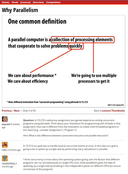
The parallel computing course in which this experiment took place met in-person twice per week for 1:20, but all lecture slides (of which there were 28 sets) were posted online. Each slide had its own discussion forum-like comments beneath it, as shown below. Students enrolled in the course were required to "individually contribute one interesting comment per lecture using the course web site" for a 5% participation grade. The experiment began in the TODO week of the course, and ran for TODO weeks.
Approximately 70 consenting students are included in this 3X2 experiment.
Voting
There were three voting conditions in this dimension: no voting, upvoting only, and downvoting, as shown below. Each student was assigned to one of these conditions, and they only ever saw one voting condition. There was the issue of cross-contamination of voting conditions, if one student looked at a peer's screen, but the instructors did not see any physical evidence of this cross contamination until the last week of the course.

Prompting
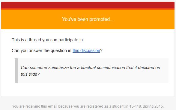
Students were also assigned to only one of two prompting conditions: positive (learning-oriented/value-emphasis) or neutral. These prompts were in the form of an email sent through the system, that would have a preset "welcome prompt" followed by a customizable "instructional prompt." The welcome prompt was either value-emphasis or neutral in tone, and the instructional prompt was either a general 'restate' request or a more specific in nature, prompting the student to answer a specific question. The welcome prompts were predefined and not customizable by the sender of the prompts, while the instructional portion was customizable. In order to maintain the utility of the email prompots, instructor-customization had to be supported.
| Neutral Welcome Prompt | Positive Welcome Prompt |
|
|
| Context - Restate (customizable) | Context - Question (customizable) |
|
|
A course instructor might decide to prompt some students to answer another students' question, as this is a valuable learning activity. When a course instructor decides to send an email prompt to a student, the system would randomly select two students. The instructor would select and customize the instructional prompt and upon submitting, the system would send an email to two students, with an appropriate version of a randomly selected welcome prompt. An example email prompt is shown below:
Processing Logfiles
Processing the logfiles mostly involves: (1) ensuring that only consenting students are included in the dataset, (2) that each comment is assigned an LDA topic, (3) that student names are removed from the dataset, (4) removing course instructors from the dataset, (5) removing spaces from column headers, and (6) removing approximately 241 comments from the logfiles that were posted to a lecture slide more than 2-3 weeks in the past (i.e., attempted cramming for an increased participation grade).
Statistical Analysis
I used the pandas and statsmodels libraries to run descriptive statistics, generate plots to better understand the data, and answer our research questions (from above). The main effects of interest were the categorical condition variables, voting (updownvote, upvote, novote) & prompts (positive, neutral) and a variety of scalar dependent variables (number of comments, comment quality, help seeking, and learning).
# necessary libraries/setup
%matplotlib inline
import utilsSPOC as utils  # separate file that contains all the constants we need
import pandas as pd
import matplotlib.pyplot as plt
# need a few more libraries for ANOVA analysis
from statsmodels.formula.api import ols
from statsmodels.stats.anova import anova_lm
# importing seaborns for its factorplot
import seaborn as sns
sns.set_style("darkgrid")
sns.set_context("notebook")

data_comments = pd.io.parsers.read_csv("150512_spoc_comments_lda.csv", encoding="utf8")
data_prompts = pd.io.parsers.read_csv("150512_spoc_prompts_mod.csv", encoding="utf8")
data = pd.io.parsers.read_csv("150512_spoc_full_data_mod.csv", encoding="utf-8-sig")
conditions = [utils.COL_VOTING, utils.COL_PROMPTS]  # all our categorical IVs of interest
covariate = utils.COL_NUM_PROMPTS  # number of prompts received needs to be controlled for
outcome = utils.COL_NUM_LEGIT_COMMENTS
Descriptive Statistics
Descriptive statistics showed that the mean number of comments students posted was 19 and the median was 17. Students also saw a mean and median number of '1' email prompts.
df = data[[covariate, outcome]]
df.describe()
# note: the log-processing removes the Prompting condition of any student who did not see a prompt
| NumTimesPrompted | num_punctual_comments | |
|---|---|---|
| count | 65.000000 | 65.000000 |
| mean | 1.169231 | 10.076923 |
| std | 1.024226 | 9.270767 |
| min | 0.000000 | 0.000000 |
| 25% | 0.000000 | 1.000000 |
| 50% | 1.000000 | 9.000000 |
| 75% | 2.000000 | 16.000000 |
| max | 5.000000 | 39.000000 |
# histogram of num comments
fig = plt.figure()
ax1 = fig.add_subplot(121)
comments_hist = data[outcome]
ax1 = comments_hist.plot(kind='hist', title="Histogram "+outcome, by=outcome)
ax1.locator_params(axis='x')
ax1.set_xlabel(outcome)
ax1.set_ylabel("Count")

ax2 = fig.add_subplot(122)
prompts_hist = data[covariate]
ax2 = prompts_hist.plot(kind='hist', title="Histogram "+covariate, by=covariate)
ax2.locator_params(axis='x')
ax2.set_xlabel(covariate)
ax2.set_ylabel("Count")

fig.tight_layout()

# plotting num prompts per day
sns.set_context("poster")
plot_prompts = data_prompts[[utils.COL_ENCOURAGEMENT_TYPE, utils.COL_TSTAMP]]
plot_prompts[utils.COL_TSTAMP] = pd.to_datetime(plot_prompts[utils.COL_TSTAMP])
plot_prompts.set_index(utils.COL_TSTAMP)
date_counts = plot_prompts[utils.COL_TSTAMP].value_counts()
date_plot = date_counts.resample('d',how=sum).plot(title="Total Prompts By Date",legend=None, kind='bar')
date_plot.set(ylim=(0, 25))
# TODO: need to find a way to drop time part of timestamp...
C:\Users\Jim\Anaconda\lib\site-packages\IPython\kernel\__main__.py:4: SettingWithCopyWarning:
A value is trying to be set on a copy of a slice from a DataFrame.
Try using .loc[row_indexer,col_indexer] = value instead

See the the caveats in the documentation: http://pandas.pydata.org/pandas-docs/stable/indexing.html#indexing-view-versus-copy
[(0, 25)]

When looking at the independent variables, we see a even random assignment to Condition. Initially, the assignment to EncouragementType wasn't perfectly even (41 vs. 27), but when we removed the prompting condition assignment of any student who did not receive any prompts, the distribution becomes more even.
df = data[conditions+[covariate, outcome]]
for cond in conditions:
    print(pd.concat([df.groupby(cond)[cond].count(), df.groupby(cond)[covariate].mean(), df.groupby(cond)[outcome].mean()], axis=1))
            Condition  NumTimesPrompted  num_punctual_comments
Condition
NOVOTE             22          1.318182              10.727273
UPDOWNVOTE         24          1.000000              10.625000
UPVOTE             19          1.210526               8.631579
                   EncouragementType  NumTimesPrompted  num_punctual_comments
EncouragementType
NEUTRAL                           25          1.400000               7.720000
NO_PROMPT                         18          0.000000              12.555556
POSITIVE                          22          1.863636              10.727273
Answering Our Research Questions
The research questions require a bit of statistics to answer. In the case of a single factor with two levels we use a t-test to determine if the independent variable in question has a significant effect on the outcome variable. In the case of a single factor with more than two levels, we use a one-way Analysis of Variance (ANOVA). With more than one factor we use a two-way ANOVA. These are all essentially similar linear models (ordinary least squares), with slightly different equations or statistics for determining significance.
What is the effect of no/up/downvoting on {learning, posting comments, posting quality comments, help seeking}
(VotingCondition --> numComments)
To answer this question, we run a one-way ANOVA (since there are more than 2 levels to this one factor). Since the p-value is above 0.05 (i.e., 0.72) we must accept the null hypothesis that there is no difference between voting conditions on number of posted comments.
cond = utils.COL_VOTING
df = data[[cond, outcome]].dropna()

cond_lm = ols(outcome + " ~ C(" + cond + ")", data=df).fit()
anova_table = anova_lm(cond_lm)
print(anova_table)
print(cond_lm.summary())

# boxplot
fig = plt.figure()
ax = fig.add_subplot(111)
ax = df.boxplot(outcome, cond, ax=plt.gca())
ax.set_xlabel(cond)
ax.set_ylabel(outcome)
fig.tight_layout()
              df       sum_sq    mean_sq        F    PR(>F)
C(Condition)   2    56.205696  28.102848  0.32003  0.727319
Residual      62  5444.409689  87.813059      NaN       NaN
                              OLS Regression Results
=================================================================================
Dep. Variable:     num_punctual_comments   R-squared:                       0.010
Model:                               OLS   Adj. R-squared:                 -0.022
Method:                    Least Squares   F-statistic:                    0.3200
Date:                   Wed, 15 Jul 2015   Prob (F-statistic):              0.727
Time:                           00:03:07   Log-Likelihood:                -236.14
No. Observations:                     65   AIC:                             478.3
Df Residuals:                         62   BIC:                             484.8
Df Model:                              2
Covariance Type:               nonrobust
==============================================================================================
                                 coef    std err          t      P>|t|      [95.0% Conf. Int.]
----------------------------------------------------------------------------------------------
Intercept                     10.7273      1.998      5.369      0.000         6.734    14.721
C(Condition)[T.UPDOWNVOTE]    -0.1023      2.766     -0.037      0.971        -5.631     5.427
C(Condition)[T.UPVOTE]        -2.0957      2.935     -0.714      0.478        -7.962     3.771
==============================================================================
Omnibus:                        6.185   Durbin-Watson:                   1.951
Prob(Omnibus):                  0.045   Jarque-Bera (JB):                6.090
Skew:                           0.749   Prob(JB):                       0.0476
Kurtosis:                       2.930   Cond. No.                         3.72
==============================================================================

Warnings:
[1] Standard Errors assume that the covariance matrix of the errors is correctly specified.

Does showing expertise information about potential helpers increase the number of helpers the student invites to her question thread?
(EncouragementType + numPrompts --> numComments)
We run an ANCOVA (since we need to control for the number of prompts each student saw) and see that the p-value is once again not significant (i.e., 0.23).
cond = utils.COL_PROMPTS
df = data[[cond, covariate, outcome]].dropna()

cond_lm = ols(outcome + " ~ C(" + cond + ") + " + covariate, data=df).fit()
anova_table = anova_lm(cond_lm)
print(anova_table)
print(cond_lm.summary())

# boxplot
fig = plt.figure()
ax = fig.add_subplot(111)
ax = df.boxplot(outcome, cond, ax=plt.gca())
ax.set_xlabel(cond)
ax.set_ylabel(outcome)
fig.tight_layout()
                      df       sum_sq     mean_sq         F    PR(>F)
C(EncouragementType)   2   258.767304  129.383652  1.512520  0.228502
NumTimesPrompted       1    23.798525   23.798525  0.278209  0.599791
Residual              61  5218.049556   85.541796       NaN       NaN
                              OLS Regression Results
=================================================================================
Dep. Variable:     num_punctual_comments   R-squared:                       0.051
Model:                               OLS   Adj. R-squared:                  0.005
Method:                    Least Squares   F-statistic:                     1.101
Date:                   Wed, 15 Jul 2015   Prob (F-statistic):              0.356
Time:                           00:03:11   Log-Likelihood:                -234.76
No. Observations:                     65   AIC:                             477.5
Df Residuals:                         61   BIC:                             486.2
Df Model:                              3
Covariance Type:               nonrobust
=====================================================================================================
                                        coef    std err          t      P>|t|      [95.0% Conf. Int.]
-----------------------------------------------------------------------------------------------------
Intercept                             6.4852      2.984      2.174      0.034         0.519    12.451
C(EncouragementType)[T.NO_PROMPT]     6.0704      3.695      1.643      0.106        -1.319    13.459
C(EncouragementType)[T.POSITIVE]      2.5983      2.813      0.924      0.359        -3.026     8.223
NumTimesPrompted                      0.8820      1.672      0.527      0.600        -2.462     4.226
==============================================================================
Omnibus:                        9.478   Durbin-Watson:                   1.841
Prob(Omnibus):                  0.009   Jarque-Bera (JB):                9.086
Skew:                           0.855   Prob(JB):                       0.0106
Kurtosis:                       3.656   Cond. No.                         7.41
==============================================================================

Warnings:
[1] Standard Errors assume that the covariance matrix of the errors is correctly specified.

Is there an interaction between voting X prompting on {learning, posting comments, posting quality comments, help seeking}
Condition X EncouragementType + numPrompts--> numComments
The OLS output shows that neither the additive model nor the interactive/multiplicative model are significant (p = 0.53 vs. p = 0.47). The AIC scores are quite similar so we'd select the one with the lower AIC score as being a better fit to the data.
col_names = [utils.COL_VOTING, utils.COL_PROMPTS, covariate, outcome]
factor_groups = data[col_names].dropna()

formula = outcome + " ~ C(" + col_names[0] + ") + C(" + col_names[1] + ") + " + covariate
formula_interaction = outcome + " ~ C(" + col_names[0] + ") * C(" + col_names[1] + ") + " + covariate

print("= = = = = = = = " + formula + " = = = = = = = =")
lm = ols(formula, data=factor_groups).fit()  # linear model: AIC 418
print(lm.summary())

print("\n= = = = = = = = " + formula_interaction + " = = = = = = = =")
lm_interaction = ols(formula_interaction, data=factor_groups).fit()  # interaction linear model: AIC 418.1
print(lm_interaction.summary())

# We can test if they're significantly different with an ANOVA (neither is sig. so not necessary)
print("= = = = = = = = = = = = = = = = = = = = = = = = = = = = = =")
print("= = " + formula + " ANOVA = = ")
print("= = vs. " + formula_interaction + " = =")
print(anova_lm(lm, lm_interaction))
= = = = = = = = num_punctual_comments ~ C(Condition) + C(EncouragementType) + NumTimesPrompted = = = = = = = =
                              OLS Regression Results
=================================================================================
Dep. Variable:     num_punctual_comments   R-squared:                       0.065
Model:                               OLS   Adj. R-squared:                 -0.014
Method:                    Least Squares   F-statistic:                    0.8260
Date:                   Wed, 15 Jul 2015   Prob (F-statistic):              0.536
Time:                           00:03:27   Log-Likelihood:                -234.27
No. Observations:                     65   AIC:                             480.5
Df Residuals:                         59   BIC:                             493.6
Df Model:                              5
Covariance Type:               nonrobust
=====================================================================================================
                                        coef    std err          t      P>|t|      [95.0% Conf. Int.]
-----------------------------------------------------------------------------------------------------
Intercept                             6.5921      3.661      1.800      0.077        -0.734    13.918
C(Condition)[T.UPDOWNVOTE]            0.4712      2.819      0.167      0.868        -5.170     6.112
C(Condition)[T.UPVOTE]               -2.1386      2.927     -0.731      0.468        -7.995     3.718
C(EncouragementType)[T.NO_PROMPT]     6.5192      3.798      1.716      0.091        -1.081    14.119
C(EncouragementType)[T.POSITIVE]      2.4994      2.841      0.880      0.383        -3.185     8.184
NumTimesPrompted                      1.0987      1.734      0.634      0.529        -2.370     4.568
==============================================================================
Omnibus:                        9.615   Durbin-Watson:                   1.904
Prob(Omnibus):                  0.008   Jarque-Bera (JB):                9.256
Skew:                           0.864   Prob(JB):                      0.00977
Kurtosis:                       3.659   Cond. No.                         8.46
==============================================================================

Warnings:
[1] Standard Errors assume that the covariance matrix of the errors is correctly specified.

= = = = = = = = num_punctual_comments ~ C(Condition) * C(EncouragementType) + NumTimesPrompted = = = = = = = =
                              OLS Regression Results
=================================================================================
Dep. Variable:     num_punctual_comments   R-squared:                       0.138
Model:                               OLS   Adj. R-squared:                 -0.003
Method:                    Least Squares   F-statistic:                    0.9754
Date:                   Wed, 15 Jul 2015   Prob (F-statistic):              0.470
Time:                           00:03:28   Log-Likelihood:                -231.66
No. Observations:                     65   AIC:                             483.3
Df Residuals:                         55   BIC:                             505.1
Df Model:                              9
Covariance Type:               nonrobust
================================================================================================================================
                                                                   coef    std err          t      P>|t|      [95.0% Conf. Int.]
--------------------------------------------------------------------------------------------------------------------------------
Intercept                                                        4.6678      4.203      1.111      0.272        -3.755    13.091
C(Condition)[T.UPDOWNVOTE]                                       4.2664      4.436      0.962      0.340        -4.624    13.157
C(Condition)[T.UPVOTE]                                           2.0318      4.808      0.423      0.674        -7.604    11.667
C(EncouragementType)[T.NO_PROMPT]                                8.1655      5.660      1.443      0.155        -3.178    19.509
C(EncouragementType)[T.POSITIVE]                                 8.5283      4.770      1.788      0.079        -1.032    18.088
C(Condition)[T.UPDOWNVOTE]:C(EncouragementType)[T.NO_PROMPT]    -0.4331      6.959     -0.062      0.951       -14.379    13.513
C(Condition)[T.UPVOTE]:C(EncouragementType)[T.NO_PROMPT]        -6.6985      7.202     -0.930      0.356       -21.131     7.734
C(Condition)[T.UPDOWNVOTE]:C(EncouragementType)[T.POSITIVE]    -10.9197      6.426     -1.699      0.095       -23.797     1.958
C(Condition)[T.UPVOTE]:C(EncouragementType)[T.POSITIVE]         -6.0041      6.955     -0.863      0.392       -19.943     7.934
NumTimesPrompted                                                 0.5548      1.749      0.317      0.752        -2.951     4.060
==============================================================================
Omnibus:                        6.251   Durbin-Watson:                   1.878
Prob(Omnibus):                  0.044   Jarque-Bera (JB):                5.391
Skew:                           0.598   Prob(JB):                       0.0675
Kurtosis:                       3.748   Cond. No.                         20.2
==============================================================================

Warnings:
[1] Standard Errors assume that the covariance matrix of the errors is correctly specified.
= = = = = = = = = = = = = = = = = = = = = = = = = = = = = =
= = num_punctual_comments ~ C(Condition) + C(EncouragementType) + NumTimesPrompted ANOVA = =
= = vs. num_punctual_comments ~ C(Condition) * C(EncouragementType) + NumTimesPrompted = =
   df_resid          ssr  df_diff     ss_diff         F    Pr(>F)
0        59  5140.763092        0         NaN       NaN       NaN
1        55  4743.521015        4  397.242076  1.151482  0.342267
# These are ANOVA tests for determining if different models are significantly different from each other.
# Although we know from the previous step that none of these are signficant, so these tests aren't necessary.
# The ANOVA output provides the F-statistics which are necessary for reporting results.
# From: http://statsmodels.sourceforge.net/devel/examples/generated/example_interactions.html

# Tests whether the LM of just Condition is significantly different from the additive LM
print("= = = = = = = = = = = = = = = = = = = = = = = = = = = = = =")
f_just_first = outcome + " ~ C(" + col_names[0] + ")"
print("= = " + f_just_first + " ANOVA = = ")
print("= = vs. " + formula + " = =")
print(anova_lm(ols(f_just_first, data=factor_groups).fit(), ols(formula, data=factor_groups).fit()))

# Testing whether the LM of just EncouragementType is significantly different from the additive LM
print("= = = = = = = = = = = = = = = = = = = = = = = = = = = = = =")
f_just_second = outcome + " ~ C(" + col_names[1] + ") + " + covariate
print("= = " + f_just_second + " = = ")
print("= = vs. " + formula + " = =")
print(anova_lm(ols(f_just_second, data=factor_groups).fit(), ols(formula, data=factor_groups).fit()))
= = = = = = = = = = = = = = = = = = = = = = = = = = = = = =
= = NumComments ~ C(Condition) ANOVA = =
= = vs. NumComments ~ C(Condition) + C(EncouragementType) + NumTimesPrompted = =
   df_resid           ssr  df_diff     ss_diff         F    Pr(>F)
0        62  17408.632376        0         NaN       NaN       NaN
1        59  16497.225960        3  911.406417  1.086505  0.361914
= = = = = = = = = = = = = = = = = = = = = = = = = = = = = =
= = NumComments ~ C(EncouragementType) + NumTimesPrompted = =
= = vs. NumComments ~ C(Condition) + C(EncouragementType) + NumTimesPrompted = =
   df_resid           ssr  df_diff    ss_diff         F    Pr(>F)
0        61  16530.305736        0        NaN       NaN       NaN
1        59  16497.225960        2  33.079776  0.059153  0.942619
# plotting
from statsmodels.graphics.api import interaction_plot
sns.set_context("notebook")

fig = plt.figure()
ax1 = sns.factorplot(x=col_names[1], y=outcome, data=factor_groups, kind='point', ci=95)
ax1.set(ylim=(0, 45))
ax2 = sns.factorplot(x=col_names[0], y=outcome, data=factor_groups, kind='point', ci=95)
ax2.set(ylim=(0, 45))
ax3 = sns.factorplot(x=col_names[1], hue=col_names[0], y=outcome, data=factor_groups, kind='point', ci=95)
ax3.set(ylim=(0, 45))
<seaborn.axisgrid.FacetGrid at 0x9d8d160>
<matplotlib.figure.Figure at 0xa2aa3c8>


This last interaction plot is interesting, and suggests that we might want to look at the "downvote" condition compared to the "non-downvote" conditions, a split which is captured in our 'COL_NEG_VOTE' column. Neither model appears significant, and an additional test shows neither model performs statistically better than the other (p = 0.1).
# sample code for calculating new column reformulation
def get_neg_vote(voting_cond)
        if voting_cond == utils.COND_VOTE_NONE or voting_cond == utils.COND_VOTE_UP:
            return utils.COND_OTHER
        elif voting_cond == utils.COND_VOTE_BOTH:
            return utils.COND_VOTE_BOTH
        else:
            return ""

# if you're missing the log processing, you can get a 'negativeVoting' column with something like this code:
data[utils.COL_NEG_VOTE] = data[utils.COL_VOTING].apply(lambda x: get_neg_vote(x))
col_names = [utils.COL_NEG_VOTE, utils.COL_PROMPTS, covariate, outcome]
factor_groups = data[col_names].dropna()

formula = outcome + " ~ C(" + col_names[0] + ") + C(" + col_names[1] + ") + " + covariate
formula_interaction = outcome + " ~ C(" + col_names[0] + ") * C(" + col_names[1] + ") + " + covariate

print("= = = = = = = = " + formula + " = = = = = = = =")
lm = ols(formula, data=factor_groups).fit()  # linear model: AIC 416
print(lm.summary())

print("\n= = = = = = = = " + formula_interaction + " = = = = = = = =")
lm_interaction = ols(formula_interaction, data=factor_groups).fit()  # interaction linear model: AIC 414
print(lm_interaction.summary())

# We can test if they're significantly different with an ANOVA (neither is sig. so not necessary)
print("= = = = = = = = = = = = = = = = = = = = = = = = = = = = = =")
print("= = " + formula + " ANOVA = = ")
print("= = vs. " + formula_interaction + " = =")
print(anova_lm(lm, lm_interaction))

# plotting
sns.set_context("notebook")
ax3 = sns.factorplot(x=col_names[1], hue=col_names[0], y=outcome, data=factor_groups, kind='point', ci=95)
ax3.set(ylim=(0, 45))
sns.set_context("poster")  # larger plots
ax4 = factor_groups.boxplot(return_type='axes', column=outcome, by=[col_names[0], col_names[1]])
= = = = = = = = num_punctual_comments ~ C(negativeVoting) + C(EncouragementType) + NumTimesPrompted = = = = = = = =
                              OLS Regression Results
=================================================================================
Dep. Variable:     num_punctual_comments   R-squared:                       0.057
Model:                               OLS   Adj. R-squared:                 -0.006
Method:                    Least Squares   F-statistic:                    0.9061
Date:                   Wed, 15 Jul 2015   Prob (F-statistic):              0.466
Time:                           00:03:48   Log-Likelihood:                -234.57
No. Observations:                     65   AIC:                             479.1
Df Residuals:                         60   BIC:                             490.0
Df Model:                              4
Covariance Type:               nonrobust
=========================================================================================================
                                            coef    std err          t      P>|t|      [95.0% Conf. Int.]
---------------------------------------------------------------------------------------------------------
Intercept                                 5.5690      3.370      1.653      0.104        -1.172    12.310
C(negativeVoting)[T.UPDOWNVOTE_GROUP]     1.4667      2.459      0.597      0.553        -3.451     6.385
C(EncouragementType)[T.NO_PROMPT]         6.4977      3.783      1.717      0.091        -1.070    14.065
C(EncouragementType)[T.POSITIVE]          2.5425      2.829      0.899      0.372        -3.117     8.202
NumTimesPrompted                          1.1174      1.727      0.647      0.520        -2.337     4.571
==============================================================================
Omnibus:                        9.249   Durbin-Watson:                   1.857
Prob(Omnibus):                  0.010   Jarque-Bera (JB):                8.876
Skew:                           0.863   Prob(JB):                       0.0118
Kurtosis:                       3.548   Cond. No.                         8.04
==============================================================================

Warnings:
[1] Standard Errors assume that the covariance matrix of the errors is correctly specified.

= = = = = = = = num_punctual_comments ~ C(negativeVoting) * C(EncouragementType) + NumTimesPrompted = = = = = = = =
                              OLS Regression Results
=================================================================================
Dep. Variable:     num_punctual_comments   R-squared:                       0.113
Model:                               OLS   Adj. R-squared:                  0.021
Method:                    Least Squares   F-statistic:                     1.233
Date:                   Wed, 15 Jul 2015   Prob (F-statistic):              0.303
Time:                           00:03:48   Log-Likelihood:                -232.57
No. Observations:                     65   AIC:                             479.1
Df Residuals:                         58   BIC:                             494.4
Df Model:                              6
Covariance Type:               nonrobust
===========================================================================================================================================
                                                                              coef    std err          t      P>|t|      [95.0% Conf. Int.]
-------------------------------------------------------------------------------------------------------------------------------------------
Intercept                                                                   5.4942      3.550      1.548      0.127        -1.612    12.601
C(negativeVoting)[T.UPDOWNVOTE_GROUP]                                       3.3447      3.788      0.883      0.381        -4.238    10.927
C(EncouragementType)[T.NO_PROMPT]                                           5.0058      4.429      1.130      0.263        -3.859    13.871
C(EncouragementType)[T.POSITIVE]                                            5.8349      3.532      1.652      0.104        -1.236    12.905
C(negativeVoting)[T.UPDOWNVOTE_GROUP]:C(EncouragementType)[T.NO_PROMPT]     2.8219      5.948      0.474      0.637        -9.084    14.728
C(negativeVoting)[T.UPDOWNVOTE_GROUP]:C(EncouragementType)[T.POSITIVE]     -8.2502      5.541     -1.489      0.142       -19.343     2.842
NumTimesPrompted                                                            0.6342      1.725      0.368      0.714        -2.819     4.087
==============================================================================
Omnibus:                        5.871   Durbin-Watson:                   1.880
Prob(Omnibus):                  0.053   Jarque-Bera (JB):                4.992
Skew:                           0.633   Prob(JB):                       0.0824
Kurtosis:                       3.493   Cond. No.                         13.4
==============================================================================

Warnings:
[1] Standard Errors assume that the covariance matrix of the errors is correctly specified.
= = = = = = = = = = = = = = = = = = = = = = = = = = = = = =
= = num_punctual_comments ~ C(negativeVoting) + C(EncouragementType) + NumTimesPrompted ANOVA = =
= = vs. num_punctual_comments ~ C(negativeVoting) * C(EncouragementType) + NumTimesPrompted = =
   df_resid          ssr  df_diff     ss_diff         F    Pr(>F)
0        60  5187.280502        0         NaN       NaN       NaN
1        58  4878.188603        2  309.091899  1.837499  0.168363


Discussion
This analysis so far has only looked at number of comments as the dependent variable, of which there does not appear to be any significant effect. However, comment quality, help seeking, and learning are all important dependent variables to examine as well. This analysis is still in progress.
Topic Modeling
I used gensim to automatically apply topics to each forum comment.
# basic descriptive statistics
data_topic = data_comments[[utils.COL_LDA]]
data_help = data_comments[[utils.COL_HELP]]

print(data_topic[utils.COL_LDA].describe())

# histogram of LDA topics
sns.set_context("notebook")
sns.factorplot(utils.COL_LDA, data=data_topic, size=6)
count               655
unique               15
top       like*hardware
freq                 73
Name: LDAtopic, dtype: object
<seaborn.axisgrid.FacetGrid at 0x9d825c0>

We can also graph the number of comments over time, and (TODO) graph these comments by topic over time.
# num comments of each topic type by date
data_topic = data_comments[[utils.COL_LDA, utils.COL_TIMESTAMP]]
data_topic[utils.COL_TIMESTAMP] = pd.to_datetime(data_topic[utils.COL_TIMESTAMP])
data_topic = data_topic.set_index(utils.COL_TIMESTAMP)
data_topic['day'] = data_topic.index.date
counts = data_topic.groupby(['day', utils.COL_LDA]).agg(len)
print(counts.tail())

# plotting
sns.set_context("poster")
data_topic = data_comments[[utils.COL_LDA, utils.COL_TIMESTAMP]]
data_topic[utils.COL_TIMESTAMP] = pd.to_datetime(data_topic[utils.COL_TIMESTAMP])
data_topic.set_index(utils.COL_TIMESTAMP)
date_counts = data_topic[utils.COL_TIMESTAMP].value_counts()
date_plot = date_counts.resample('d',how=sum).plot(title="Total Comments By Date",legend=None)
date_plot.set(ylim=(0, 100))
C:\Users\Jim\Anaconda\lib\site-packages\IPython\kernel\__main__.py:3: SettingWithCopyWarning:
A value is trying to be set on a copy of a slice from a DataFrame.
Try using .loc[row_indexer,col_indexer] = value instead

See the the caveats in the documentation: http://pandas.pydata.org/pandas-docs/stable/indexing.html#indexing-view-versus-copy
  app.launch_new_instance()
C:\Users\Jim\Anaconda\lib\site-packages\IPython\kernel\__main__.py:12: SettingWithCopyWarning:
A value is trying to be set on a copy of a slice from a DataFrame.
Try using .loc[row_indexer,col_indexer] = value instead

See the the caveats in the documentation: http://pandas.pydata.org/pandas-docs/stable/indexing.html#indexing-view-versus-copy
day         LDAtopic
2015-05-02  will*can         1
2015-05-03  case*larger      1
2015-05-04  better*always    1
            will*can         1
2015-05-08  like*hardware    1
dtype: int64
[(0, 100)]

Research Questions
Basic descriptive statistics and bar graphs are simple enough to acquire, but what we might want to know is what topic is the most popular to write about and what topic are students requesting the most help on? To do this, we need to find out how many comments there are on a particular comment, and how many of these comments are help requests.
def count_instances(df,uid,column):
    """
    Return dataframe of total counts for each unique value in COLUMN, by UID
    :param df: the dataframe containing the data of interest
    :param uid: the unique index/ID to group the counts by (i.e., author user id)
    :param column: the column containing the things to count (i.e., help requests)
    :return: True if the string contains the letter 'y'
    """
    df['tot_comments'] = 1
    for item in df[column].unique():
        colname = "help_requests" if item == "True" else "other_comments"
        df['num_%s' % colname] = df[column].apply(lambda value: 1 if value == str(item) else 0)

    new_data = df.groupby(uid).sum()

    """#calculating percents
    cols = [col for col in new_data.columns if 'num' in col]
    for col in cols:
        new_data[col.replace('num','percent')] = new_data[col] / new_data['tot_comments'] * 100
    """
    return new_data

data_topic = data_comments[[utils.COL_LDA, utils.COL_TIMESTAMP, utils.COL_HELP]]

df_by_topic = count_instances(data_topic, utils.COL_LDA, utils.COL_HELP)  # calculate number help requests per topic

data_help = data_comments[[utils.COL_ID, utils.COL_HELP]]
data_help[utils.COL_HELP] = data_help[utils.COL_HELP].astype('str')
df_help_counts = count_instances(data_help, utils.COL_ID, utils.COL_HELP)  # calculate number help requests per user

# merging our help counts table with original data
data[utils.COL_ID] = data[utils.COL_ID].astype('str')
indexed_data = data.set_index([utils.COL_ID])
combined_df = pd.concat([indexed_data, df_help_counts], axis=1, join_axes=[indexed_data.index])

# Replace NaN in help_requests/other_comments cols with '0'
combined_df["num_help_requests"].fillna(value=0, inplace=True)
combined_df["num_other_comments"].fillna(value=0, inplace=True)
C:\Users\Jim\Anaconda\lib\site-packages\IPython\kernel\__main__.py:9: SettingWithCopyWarning:
A value is trying to be set on a copy of a slice from a DataFrame.
Try using .loc[row_indexer,col_indexer] = value instead

See the the caveats in the documentation: http://pandas.pydata.org/pandas-docs/stable/indexing.html#indexing-view-versus-copy
C:\Users\Jim\Anaconda\lib\site-packages\IPython\kernel\__main__.py:12: SettingWithCopyWarning:
A value is trying to be set on a copy of a slice from a DataFrame.
Try using .loc[row_indexer,col_indexer] = value instead

See the the caveats in the documentation: http://pandas.pydata.org/pandas-docs/stable/indexing.html#indexing-view-versus-copy
C:\Users\Jim\Anaconda\lib\site-packages\IPython\kernel\__main__.py:28: SettingWithCopyWarning:
A value is trying to be set on a copy of a slice from a DataFrame.
Try using .loc[row_indexer,col_indexer] = value instead

See the the caveats in the documentation: http://pandas.pydata.org/pandas-docs/stable/indexing.html#indexing-view-versus-copy
Help Seeking
I used an extremely naive set of rules to determine if a comment was a help request, such as identifying if a question mark is included in the message (or the word 'question', or 'struggle' or 'stuck', etc) I identified which entries are most likely help requests and which are not. In the future, a coding scheme should be developed to determine what kinds of help are being sought.
# example code - does not need to execute
def is_help_topic(sentence):
    if "help" in sentence or "question" in sentence or "?" in sentence or "dunno" in sentence or "n't know" in sentence:
        return True
    if "confus" in sentence or "struggl" in sentence or "lost" in sentence or "stuck" in sentence or "know how" in sentence:
        return True
    return False

# if you're missing the log processing, you can get an 'isHelpSeeking' column with something like this code:
data_comments[utils.COL_HELP] = data_comments[utils.COL_COMMENT].apply(lambda x: is_help_topic(x))
# histogram of help requests
sns.factorplot(utils.COL_HELP, data=data_help, size=6)
data_help.describe()

# plotting
"""
sns.set_context("poster")
data_by_date = data[[utils.COL_HELP, utils.COL_TIMESTAMP]]
data_by_date[utils.COL_TIMESTAMP] = pd.to_datetime(data_by_date[utils.COL_TIMESTAMP])
data_by_date.set_index(utils.COL_TIMESTAMP)
date_counts = data_by_date[utils.COL_TIMESTAMP].value_counts()
date_plot = date_counts.resample('d',how=sum).plot(title="Total Help Requests By Date",legend=None)
date_plot.set(ylim=(0, 100))
"""
'\nsns.set_context("poster")\ndata_by_date = data[[utils.COL_HELP, utils.COL_TIMESTAMP]]\ndata_by_date[utils.COL_TIMESTAMP] = pd.to_datetime(data_by_date[utils.COL_TIMESTAMP])\ndata_by_date.set_index(utils.COL_TIMESTAMP)\ndate_counts = data_by_date[utils.COL_TIMESTAMP].value_counts()\ndate_plot = date_counts.resample(\'d\',how=sum).plot(title="Total Help Requests By Date",legend=None)\ndate_plot.set(ylim=(0, 100))\n'

Now, instead of using 'numComments' as our outcome variable, we can use 'numHelpRequests' as the outcome variable. But first we have to calculate that for each user.
data_help = data_comments[[utils.COL_AUTHOR, utils.COL_HELP]]
data_help.rename(columns={utils.COL_AUTHOR:utils.COL_ID}, inplace=True)  #rename so we can merge later
data_help[utils.COL_ID] = data_help[utils.COL_ID].astype('str')
data_help[utils.COL_HELP] = data_help[utils.COL_HELP].astype('str')

# merging our help counts table with original data
df_help_counts.drop("tot_comments", axis=1, inplace=True)
data[utils.COL_ID] = data[utils.COL_ID].astype('str')
indexed_data = data.set_index([utils.COL_ID])
combined_df = pd.concat([indexed_data, df_help_counts], axis=1, join_axes=[indexed_data.index])

# Replace NaN in help_requests/other_comments cols with '0'
combined_df["num_help_requests"].fillna(value=0, inplace=True)
combined_df["num_other_comments"].fillna(value=0, inplace=True)
C:\Users\Jim\Anaconda\lib\site-packages\IPython\kernel\__main__.py:3: SettingWithCopyWarning:
A value is trying to be set on a copy of a slice from a DataFrame.
Try using .loc[row_indexer,col_indexer] = value instead

See the the caveats in the documentation: http://pandas.pydata.org/pandas-docs/stable/indexing.html#indexing-view-versus-copy
  app.launch_new_instance()
C:\Users\Jim\Anaconda\lib\site-packages\IPython\kernel\__main__.py:4: SettingWithCopyWarning:
A value is trying to be set on a copy of a slice from a DataFrame.
Try using .loc[row_indexer,col_indexer] = value instead

See the the caveats in the documentation: http://pandas.pydata.org/pandas-docs/stable/indexing.html#indexing-view-versus-copy
---------------------------------------------------------------------------
ValueError                                Traceback (most recent call last)
<ipython-input-18-3eb8b6e3ae09> in <module>()
      5
      6 # merging our help counts table with original data
----> 7 df_help_counts.drop("tot_comments", axis=1, inplace=True)
      8 data[utils.COL_ID] = data[utils.COL_ID].astype('str')
      9 indexed_data = data.set_index([utils.COL_ID])

C:\Users\Jim\Anaconda\lib\site-packages\pandas\core\generic.py in drop(self, labels, axis, level, inplace)
   1584                 new_axis = axis.drop(labels, level=level)
   1585             else:
-> 1586                 new_axis = axis.drop(labels)
   1587             dropped = self.reindex(**{axis_name: new_axis})
   1588             try:

C:\Users\Jim\Anaconda\lib\site-packages\pandas\core\index.py in drop(self, labels)
   2342         mask = indexer == -1
   2343         if mask.any():
-> 2344             raise ValueError('labels %s not contained in axis' % labels[mask])
   2345         return self.delete(indexer)
   2346

ValueError: labels ['tot_comments'] not contained in axis
outcome = "num_help_requests"
col_names = [utils.COL_NEG_VOTE, utils.COL_PROMPTS, covariate, outcome]
factor_groups = combined_df[col_names].dropna()

formula = outcome + " ~ C(" + col_names[0] + ") + C(" + col_names[1] + ") + " + covariate
formula_interaction = outcome + " ~ C(" + col_names[0] + ") * C(" + col_names[1] + ") + " + covariate

print("= = = = = = = = " + formula + " = = = = = = = =")
lm = ols(formula, data=factor_groups).fit()  # linear model: AIC 416
print(lm.summary())

print("\n= = = = = = = = " + formula_interaction + " = = = = = = = =")
lm_interaction = ols(formula_interaction, data=factor_groups).fit()  # interaction linear model: AIC 414
print(lm_interaction.summary())

# We can test if they're significantly different with an ANOVA (neither is sig. so not necessary)
print("= = = = = = = = = = = = = = = = = = = = = = = = = = = = = =")
print("= = " + formula + " ANOVA = = ")
print("= = vs. " + formula_interaction + " = =")
print(anova_lm(lm, lm_interaction))

# plotting
sns.set_context("notebook")
ax3 = sns.factorplot(x=col_names[1], hue=col_names[0], y=outcome, data=factor_groups, kind='point', ci=95)
ax3.set(ylim=(0, 45))
sns.set_context("poster")  # larger plots
ax4 = factor_groups.boxplot(return_type='axes', column=outcome, by=[col_names[0], col_names[1]])
= = = = = = = = num_help_requests ~ C(negativeVoting) + C(EncouragementType) + NumTimesPrompted = = = = = = = =
---------------------------------------------------------------------------
ValueError                                Traceback (most recent call last)
<ipython-input-17-64db1f3c8af3> in <module>()
      7
      8 print("= = = = = = = = " + formula + " = = = = = = = =")
----> 9 lm = ols(formula, data=factor_groups).fit()  # linear model: AIC 416
     10 print(lm.summary())
     11

C:\Users\Jim\Anaconda\lib\site-packages\statsmodels\base\model.py in from_formula(cls, formula, data, subset, *args, **kwargs)
    145         (endog, exog), missing_idx = handle_formula_data(data, None, formula,
    146                                                          depth=eval_env,
--> 147                                                          missing=missing)
    148         kwargs.update({'missing_idx': missing_idx,
    149                        'missing': missing})

C:\Users\Jim\Anaconda\lib\site-packages\statsmodels\formula\formulatools.py in handle_formula_data(Y, X, formula, depth, missing)
     63         if data_util._is_using_pandas(Y, None):
     64             result = dmatrices(formula, Y, depth, return_type='dataframe',
---> 65                                NA_action=na_action)
     66         else:
     67             result = dmatrices(formula, Y, depth, return_type='dataframe',

C:\Users\Jim\Anaconda\lib\site-packages\patsy\highlevel.py in dmatrices(formula_like, data, eval_env, NA_action, return_type)
    295     eval_env = EvalEnvironment.capture(eval_env, reference=1)
    296     (lhs, rhs) = _do_highlevel_design(formula_like, data, eval_env,
--> 297                                       NA_action, return_type)
    298     if lhs.shape[1] == 0:
    299         raise PatsyError("model is missing required outcome variables")

C:\Users\Jim\Anaconda\lib\site-packages\patsy\highlevel.py in _do_highlevel_design(formula_like, data, eval_env, NA_action, return_type)
    150         return iter([data])
    151     builders = _try_incr_builders(formula_like, data_iter_maker, eval_env,
--> 152                                   NA_action)
    153     if builders is not None:
    154         return build_design_matrices(builders, data,

C:\Users\Jim\Anaconda\lib\site-packages\patsy\highlevel.py in _try_incr_builders(formula_like, data_iter_maker, eval_env, NA_action)
     55                                        formula_like.rhs_termlist],
     56                                       data_iter_maker,
---> 57                                       NA_action)
     58     else:
     59         return None

C:\Users\Jim\Anaconda\lib\site-packages\patsy\build.py in design_matrix_builders(termlists, data_iter_maker, NA_action)
    678         result = _make_term_column_builders(termlist,
    679                                             num_column_counts,
--> 680                                             cat_levels_contrasts)
    681         new_term_order, term_to_column_builders = result
    682         assert frozenset(new_term_order) == frozenset(termlist)

C:\Users\Jim\Anaconda\lib\site-packages\patsy\build.py in _make_term_column_builders(terms, num_column_counts, cat_levels_contrasts)
    607                         coded = code_contrast_matrix(factor_coding[factor],
    608                                                      levels, contrast,
--> 609                                                      default=Treatment)
    610                         cat_contrasts[factor] = coded
    611                 column_builder = _ColumnBuilder(builder_factors,

C:\Users\Jim\Anaconda\lib\site-packages\patsy\contrasts.py in code_contrast_matrix(intercept, levels, contrast, default)
    574         return contrast.code_with_intercept(levels)
    575     else:
--> 576         return contrast.code_without_intercept(levels)
    577

C:\Users\Jim\Anaconda\lib\site-packages\patsy\contrasts.py in code_without_intercept(self, levels)
    170         else:
    171             reference = _get_level(levels, self.reference)
--> 172         eye = np.eye(len(levels) - 1)
    173         contrasts = np.vstack((eye[:reference, :],
    174                                 np.zeros((1, len(levels) - 1)),

C:\Users\Jim\Anaconda\lib\site-packages\numpy\lib\twodim_base.py in eye(N, M, k, dtype)
    229     if M is None:
    230         M = N
--> 231     m = zeros((N, M), dtype=dtype)
    232     if k >= M:
    233         return m

ValueError: negative dimensions are not allowed
Conclusion
In conclusion, ...TODO: there's still more analysis to do...