Neural network methods
Author: Gaurav Vaidya
Learning objectives
- Understand what an artificial neural network (ANN) is and how it can be used.
- Implement ANNs for use in prediction and classification based on multiple input features.
Learning deeply
Artificial Neural Networks (ANNs) and deep learning are currently getting a lot of interest, both as a subject of research and as a tool for analyzing datasets. A big difference from other machine learning techniques we've looked at so far is that ANNs can identify characteristics of interest by themselves, rather than having to be chosen by data scientists. Some of the other advantages of ANNs are related specifically to interpreting video and audio data, such as by using convolutional neural networks, but today we will focus on simple ANNs so you understand their struction and function.
Units
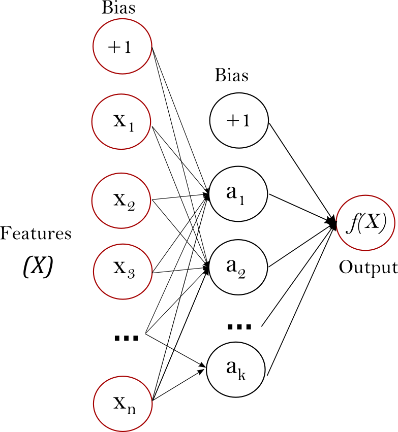
ANNs are designed as layers of units (or nodes, or artificial neurons). Each unit accepts multiple inputs, each of which has a different weight, including one bias input, which it combines into a single value. That single value is passed to an activation function, which provides an output only if the combined value is greater than a particular threshold (usually, zero).
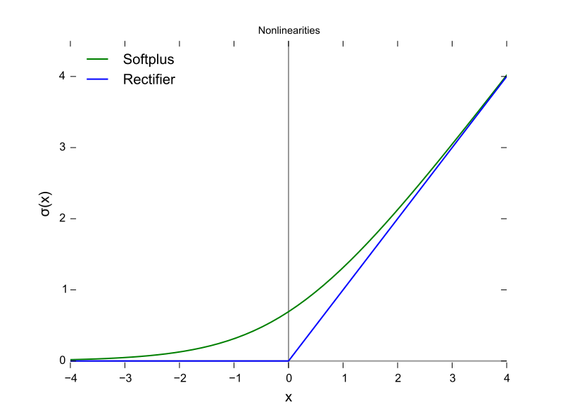
In effect, each unit focuses on a particular aspect of the layer underneath it, and then summarizing that information for the layer above it. Every input to every unit has a weight and the unit has a bias input, and so is effectively doing a linear regression on the incoming data to obtain an output. The use of a non-linear activation function allows the ANN to predict and classify data that are not linearly separable. ANNs used to use the same sigmoid function we saw before, but these days the rectified linear unit (ReLU) function has become much more popular. It simply returns zero when the real output value is less than zero.
Layers
Every neural network has three layers:
- An input layer, where each unit corresponds to a particular input feature. This could be categorical data, continuous data, or even colour values from images.
- An output layer. We will be running two examples today: in the first, we will use a single output unit (the predicted price for a particular house in California). In the second, we will use seven output units, each corresponding to a particular type of forest cover.
- A hidden layer. Without a hidden layer, an ANN can only pick up linear relationships: how changes in the input layer correspond to values in the output layer. Thanks to the hidden layer, an ANN can also pick up non-linear relationships, where different groups of input values interact in complicated ways to get the correct response on the output layer. The "deep" in deep learning refers to the hidden layers that allow the model to identify intermediate patterns between the input and output layers.
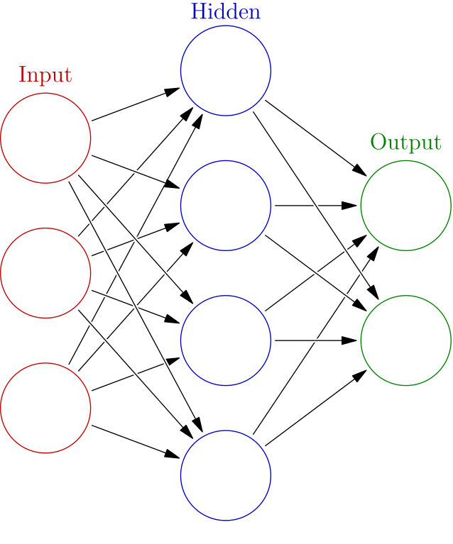
Putting it all together, we end up with a type of ANN called a multilayer perceptron (MLP) network, which looks like the following:
Google's Machine Learning course puts this very nicely: "Stacking nonlinearities on nonlinearities lets us model very complicated relationships between the inputs and the predicted outputs. In brief, each layer is effectively learning a more complex, higher-level function over the raw inputs."
So what do we need?
To create an ANN, we need to choose:
- The number of input units (= the number of input features)
- The number of output units:
- When using the ANN to predict, we generally only need a single output unit.
- When using the ANN to classify, we generally set the number of output units to the number of possible labels.
- The number of hidden layers
- More hidden layers allows for more complex models -- which, as you've learned, also increases your risk of overfitting! So you want to go for the simplest model that meets your needs.
- A loss function. The scikit-learn classes we use always use logistic loss, also known as cross-entropy loss.
- The solver to use. The solver controls learning by searching for local minima in the parameter space. ANNs generally use stochastic gradient descent (SGD) such as RMSProp, but today we will use Adaptive Moment Estimation (Adam).
- The regularization protocol. We will use L2 regularization.
Note that these are the hyperparameters of our model: we will adjust these hyperparameters to improve how quickly and accurately we can determine the actual parameters of our model, which is the set of weights and biases on all units across all layers.
Reminders of the ground rules
- Always have training data and testing data, and make sure the ANN never sees the testing data.
- Always shuffle your data.
- ANNs don't work well when the features are in different ranges: it's usually a good idea to normalize it before use.
ANN for prediction: how much might this house cost?
There aren't very good datasets for showcasing prediction on biological data, so we will use one of the classic machine learning datasets: a dataset of California house prices, based on the 1990 census and published in Pace and Barry, 1997. Scikit-Learn can download this dataset for us, so let's start with that.
from sklearn import datasets
help(datasets.fetch_california_housing)
Help on function fetch_california_housing in module sklearn.datasets.california_housing:

fetch_california_housing(data_home=None, download_if_missing=True, return_X_y=False)
    Load the California housing dataset (regression).

    ==============     ==============
    Samples total               20640
    Dimensionality                  8
    Features                     real
    Target             real 0.15 - 5.
    ==============     ==============

    Read more in the :ref:`User Guide <california_housing_dataset>`.

    Parameters
    ----------
    data_home : optional, default: None
        Specify another download and cache folder for the datasets. By default
        all scikit-learn data is stored in '~/scikit_learn_data' subfolders.

    download_if_missing : optional, default=True
        If False, raise a IOError if the data is not locally available
        instead of trying to download the data from the source site.


    return_X_y : boolean, default=False.
        If True, returns ``(data.data, data.target)`` instead of a Bunch
        object.

        .. versionadded:: 0.20

    Returns
    -------
    dataset : dict-like object with the following attributes:

    dataset.data : ndarray, shape [20640, 8]
        Each row corresponding to the 8 feature values in order.

    dataset.target : numpy array of shape (20640,)
        Each value corresponds to the average house value in units of 100,000.

    dataset.feature_names : array of length 8
        Array of ordered feature names used in the dataset.

    dataset.DESCR : string
        Description of the California housing dataset.

    (data, target) : tuple if ``return_X_y`` is True

        .. versionadded:: 0.20

    Notes
    ------

    This dataset consists of 20,640 samples and 9 features.
import numpy as np
import pandas as pd

# Fetch California housing dataset. This will be downloaded to your computer.
calif = datasets.fetch_california_housing()
print("Shape of California housing data: ", calif.data.shape)
califdf = pd.DataFrame.from_records(calif.data, columns=calif.feature_names)
califdf.head()
Shape of California housing data: (20640, 8)
| MedInc | HouseAge | AveRooms | AveBedrms | Population | AveOccup | Latitude | Longitude | |
|---|---|---|---|---|---|---|---|---|
| 0 | 8.3252 | 41.0 | 6.984127 | 1.023810 | 322.0 | 2.555556 | 37.88 | -122.23 |
| 1 | 8.3014 | 21.0 | 6.238137 | 0.971880 | 2401.0 | 2.109842 | 37.86 | -122.22 |
| 2 | 7.2574 | 52.0 | 8.288136 | 1.073446 | 496.0 | 2.802260 | 37.85 | -122.24 |
| 3 | 5.6431 | 52.0 | 5.817352 | 1.073059 | 558.0 | 2.547945 | 37.85 | -122.25 |
| 4 | 3.8462 | 52.0 | 6.281853 | 1.081081 | 565.0 | 2.181467 | 37.85 | -122.25 |
# What do the house prices look like?
print(calif.target[0:5]) # Units: $100,000x
[4.526 3.585 3.521 3.413 3.422]
Let's start by shuffling our data and splitting into testing data and training data.
from sklearn import model_selection
X_train, X_test, y_train, y_test = model_selection.train_test_split(
    califdf,        # Input features (X)
    calif.target,   # Output features (y)
    test_size=0.25, # Put aside 25% of data for testing.
    shuffle=True    # Shuffle inputs.
)

# Did we err?

print("Train data shape: ", X_train.shape)
print("Train label shape: ", y_train.shape)

print("Test data shape: ", X_test.shape)
print("Test label shape: ", y_test.shape)
Train data shape:  (15480, 8)
Train label shape:  (15480,)
Test data shape:  (5160, 8)
Test label shape:  (5160,)
# Let's have a look at the data. Is it in similar ranges?
import pandas as pd
pd.DataFrame(X_train).describe()
| MedInc | HouseAge | AveRooms | AveBedrms | Population | AveOccup | Latitude | Longitude | |
|---|---|---|---|---|---|---|---|---|
| count | 15480.000000 | 15480.000000 | 15480.000000 | 15480.000000 | 15480.000000 | 15480.000000 | 15480.000000 | 15480.000000 |
| mean | 3.862124 | 28.641667 | 5.421070 | 1.095826 | 1424.529134 | 2.991342 | 35.632852 | -119.577271 |
| std | 1.895399 | 12.616185 | 2.556300 | 0.491132 | 1141.545612 | 4.972682 | 2.134506 | 2.003396 |
| min | 0.499900 | 1.000000 | 0.846154 | 0.375000 | 5.000000 | 0.692308 | 32.540000 | -124.250000 |
| 25% | 2.556200 | 18.000000 | 4.433867 | 1.005435 | 788.000000 | 2.432607 | 33.930000 | -121.810000 |
| 50% | 3.533800 | 29.000000 | 5.225013 | 1.048433 | 1164.000000 | 2.821744 | 34.260000 | -118.500000 |
| 75% | 4.737500 | 37.000000 | 6.041504 | 1.099476 | 1722.000000 | 3.283372 | 37.710000 | -118.020000 |
| max | 15.000100 | 52.000000 | 141.909091 | 34.066667 | 35682.000000 | 599.714286 | 41.950000 | -114.310000 |
The input data comes in many different ranges: compare the ranges of latitude (32.54 to 41.95), longitude (-124.35 to -114.31), median income (0.50 to 15.0) and population (3 to 35682). As we described earlier, it's a good idea to normalize these values. Scikit-Learn has several built-in scalers that do just this. We will use the StandardScaler, which changes the data so it is normally distributed, with a mean of 0 and a variance of 1, but other standardization methods are available.
from sklearn.preprocessing import StandardScaler

scaler = StandardScaler()

# Figure out how to scale all the input features in the training dataset.
scaler.fit(X_train)
X_train_scaled = scaler.transform(X_train)

# Also tranform our validation and testing data in the same way.
X_test_scaled = scaler.transform(X_test)

# Did that work?
pd.DataFrame(X_train_scaled).describe()
| 0 | 1 | 2 | 3 | 4 | 5 | 6 | 7 | |
|---|---|---|---|---|---|---|---|---|
| count | 1.548000e+04 | 1.548000e+04 | 1.548000e+04 | 1.548000e+04 | 1.548000e+04 | 1.548000e+04 | 1.548000e+04 | 1.548000e+04 |
| mean | -1.468822e-16 | 7.527714e-17 | 1.383906e-16 | 3.442552e-17 | 2.754042e-18 | 4.039261e-17 | -6.334296e-16 | -3.809758e-16 |
| std | 1.000032e+00 | 1.000032e+00 | 1.000032e+00 | 1.000032e+00 | 1.000032e+00 | 1.000032e+00 | 1.000032e+00 | 1.000032e+00 |
| min | -1.773945e+00 | -2.191040e+00 | -1.789721e+00 | -1.467731e+00 | -1.243555e+00 | -4.623478e-01 | -1.449025e+00 | -2.332479e+00 |
| 25% | -6.890194e-01 | -8.435205e-01 | -3.861969e-01 | -1.840523e-01 | -5.576209e-01 | -1.123645e-01 | -7.977993e-01 | -1.114508e+00 |
| 50% | -1.732274e-01 | 2.840359e-02 | -7.669808e-02 | -9.650046e-02 | -2.282323e-01 | -3.410707e-02 | -6.431918e-01 | 5.377399e-01 |
| 75% | 4.618574e-01 | 6.625302e-01 | 2.427153e-01 | 7.433478e-03 | 2.605945e-01 | 5.872883e-02 | 9.731598e-01 | 7.773408e-01 |
| max | 5.876513e+00 | 1.851518e+00 | 5.339453e+01 | 6.713457e+01 | 3.001070e+01 | 1.200041e+02 | 2.959632e+00 | 2.629256e+00 |
We won't normalize the output labels for simplicity and because it's usually not necessary if you have a single output. However, if you have multiple output labels, you will want to normalize them to each other.
Alright, we're ready to run our model! We will use the MLPRegressor -- MLP stands for multilevel perceptron, a description of this kind of neural network.
from sklearn.neural_network import MLPRegressor

ann = MLPRegressor(
    activation='relu',  # The activation function to use: ReLU
    solver='adam',      # The solver to use
    alpha=0.001,        # The L2 regularization rate: higher values increase cost for larger weights
    hidden_layer_sizes=(50, 20),
                        # The number of units in each hidden layer.
                        # Note that we don't need to specify input and output neuron numbers:
                        # MLPClassifier determines this based on the shape of the features and labels
                        # being fitted.
    verbose=True,       # Report on progress.
    batch_size='auto',  # Process dataset in batches of 200 rows at a time.
    early_stopping=True # This activates two features:
                        #  - We will hold 10% of data aside as validation data. At the end of each
                        #    iteration, we will test the validation data to see how well we're doing.
                        #  - If learning slows below a pre-determined level, we stop early rather than
                        #    overtraining on our data.
)
ann.fit(X_train_scaled, y_train)
Iteration 1, loss = 1.78395319
Validation score: 0.269671
Iteration 2, loss = 0.40048710
Validation score: 0.496960
Iteration 3, loss = 0.30416513
Validation score: 0.568650
Iteration 4, loss = 0.26045892
Validation score: 0.611116
Iteration 5, loss = 0.23380253
Validation score: 0.641203
Iteration 6, loss = 0.21744966
Validation score: 0.659125
Iteration 7, loss = 0.20602815
Validation score: 0.671523
Iteration 8, loss = 0.19877348
Validation score: 0.677612
Iteration 9, loss = 0.19326475
Validation score: 0.684275
Iteration 10, loss = 0.18926257
Validation score: 0.690023
Iteration 11, loss = 0.18622392
Validation score: 0.693421
Iteration 12, loss = 0.18364689
Validation score: 0.696335
Iteration 13, loss = 0.18100021
Validation score: 0.702679
Iteration 14, loss = 0.17879836
Validation score: 0.705411
Iteration 15, loss = 0.17674397
Validation score: 0.707982
Iteration 16, loss = 0.17475785
Validation score: 0.709925
Iteration 17, loss = 0.17325396
Validation score: 0.712813
Iteration 18, loss = 0.17186204
Validation score: 0.714069
Iteration 19, loss = 0.17057713
Validation score: 0.718573
Iteration 20, loss = 0.16939444
Validation score: 0.716752
Iteration 21, loss = 0.16808567
Validation score: 0.722229
Iteration 22, loss = 0.16696640
Validation score: 0.721332
Iteration 23, loss = 0.16616058
Validation score: 0.725791
Iteration 24, loss = 0.16496505
Validation score: 0.724879
Iteration 25, loss = 0.16343029
Validation score: 0.728570
Iteration 26, loss = 0.16266397
Validation score: 0.728714
Iteration 27, loss = 0.16140440
Validation score: 0.733954
Iteration 28, loss = 0.15990542
Validation score: 0.732648
Iteration 29, loss = 0.15905258
Validation score: 0.737474
Iteration 30, loss = 0.15700726
Validation score: 0.736568
Iteration 31, loss = 0.15603395
Validation score: 0.740053
Iteration 32, loss = 0.15512096
Validation score: 0.739522
Iteration 33, loss = 0.15510144
Validation score: 0.739999
Iteration 34, loss = 0.15324322
Validation score: 0.743014
Iteration 35, loss = 0.15267468
Validation score: 0.744724
Iteration 36, loss = 0.15275319
Validation score: 0.746584
Iteration 37, loss = 0.15069781
Validation score: 0.745608
Iteration 38, loss = 0.15100557
Validation score: 0.746861
Iteration 39, loss = 0.14962103
Validation score: 0.748189
Iteration 40, loss = 0.14930208
Validation score: 0.748062
Iteration 41, loss = 0.14768952
Validation score: 0.752246
Iteration 42, loss = 0.14709483
Validation score: 0.750436
Iteration 43, loss = 0.14619772
Validation score: 0.754742
Iteration 44, loss = 0.14698924
Validation score: 0.753296
Iteration 45, loss = 0.14502456
Validation score: 0.757108
Iteration 46, loss = 0.14455279
Validation score: 0.754906
Iteration 47, loss = 0.14357148
Validation score: 0.756072
Iteration 48, loss = 0.14328472
Validation score: 0.754611
Iteration 49, loss = 0.14265293
Validation score: 0.759212
Iteration 50, loss = 0.14184246
Validation score: 0.761116
Iteration 51, loss = 0.14245981
Validation score: 0.762705
Iteration 52, loss = 0.14170275
Validation score: 0.760689
Iteration 53, loss = 0.14162699
Validation score: 0.762154
Iteration 54, loss = 0.14181699
Validation score: 0.760913
Iteration 55, loss = 0.14113317
Validation score: 0.761710
Iteration 56, loss = 0.14059386
Validation score: 0.757093
Iteration 57, loss = 0.14002683
Validation score: 0.763510
Iteration 58, loss = 0.13988032
Validation score: 0.762324
Iteration 59, loss = 0.13886572
Validation score: 0.762611
Iteration 60, loss = 0.13948545
Validation score: 0.760565
Iteration 61, loss = 0.13796855
Validation score: 0.764551
Iteration 62, loss = 0.13749400
Validation score: 0.761634
Iteration 63, loss = 0.13776950
Validation score: 0.762150
Iteration 64, loss = 0.13747980
Validation score: 0.760548
Iteration 65, loss = 0.13769208
Validation score: 0.762841
Iteration 66, loss = 0.13705944
Validation score: 0.760266
Iteration 67, loss = 0.13760656
Validation score: 0.763218
Iteration 68, loss = 0.13663838
Validation score: 0.765209
Iteration 69, loss = 0.13600413
Validation score: 0.762145
Iteration 70, loss = 0.13653847
Validation score: 0.760569
Iteration 71, loss = 0.13724037
Validation score: 0.761683
Iteration 72, loss = 0.13620033
Validation score: 0.766285
Iteration 73, loss = 0.13539298
Validation score: 0.761398
Iteration 74, loss = 0.13654450
Validation score: 0.765581
Iteration 75, loss = 0.13572818
Validation score: 0.764635
Iteration 76, loss = 0.13481307
Validation score: 0.765610
Iteration 77, loss = 0.13539711
Validation score: 0.763212
Iteration 78, loss = 0.13486477
Validation score: 0.766516
Iteration 79, loss = 0.13455420
Validation score: 0.764574
Iteration 80, loss = 0.13329891
Validation score: 0.765145
Iteration 81, loss = 0.13359457
Validation score: 0.761580
Iteration 82, loss = 0.13324071
Validation score: 0.767093
Iteration 83, loss = 0.13334167
Validation score: 0.768302
Iteration 84, loss = 0.13305772
Validation score: 0.765975
Iteration 85, loss = 0.13302991
Validation score: 0.765658
Iteration 86, loss = 0.13235215
Validation score: 0.768617
Iteration 87, loss = 0.13205636
Validation score: 0.762191
Iteration 88, loss = 0.13251709
Validation score: 0.767893
Iteration 89, loss = 0.13216362
Validation score: 0.764732
Iteration 90, loss = 0.13183369
Validation score: 0.769772
Iteration 91, loss = 0.13174595
Validation score: 0.769393
Iteration 92, loss = 0.13176786
Validation score: 0.769545
Iteration 93, loss = 0.13167039
Validation score: 0.767980
Iteration 94, loss = 0.13133042
Validation score: 0.764848
Iteration 95, loss = 0.13721522
Validation score: 0.766268
Iteration 96, loss = 0.13296603
Validation score: 0.770427
Iteration 97, loss = 0.13028083
Validation score: 0.766183
Iteration 98, loss = 0.13026281
Validation score: 0.768261
Iteration 99, loss = 0.12995922
Validation score: 0.771497
Iteration 100, loss = 0.13009093
Validation score: 0.770901
Iteration 101, loss = 0.12921611
Validation score: 0.773096
Iteration 102, loss = 0.12937084
Validation score: 0.771619
Iteration 103, loss = 0.12943766
Validation score: 0.768302
Iteration 104, loss = 0.12919797
Validation score: 0.773403
Iteration 105, loss = 0.12894905
Validation score: 0.771725
Iteration 106, loss = 0.13001117
Validation score: 0.773794
Iteration 107, loss = 0.12871301
Validation score: 0.769237
Iteration 108, loss = 0.12970825
Validation score: 0.771186
Iteration 109, loss = 0.12829932
Validation score: 0.771517
Iteration 110, loss = 0.12854296
Validation score: 0.773027
Iteration 111, loss = 0.12832205
Validation score: 0.773978
Iteration 112, loss = 0.12837127
Validation score: 0.769361
Iteration 113, loss = 0.13116502
Validation score: 0.772059
Iteration 114, loss = 0.12819269
Validation score: 0.772295
Iteration 115, loss = 0.12759859
Validation score: 0.769477
Iteration 116, loss = 0.12792852
Validation score: 0.771334
Iteration 117, loss = 0.12850087
Validation score: 0.772960
Iteration 118, loss = 0.12810867
Validation score: 0.772603
Iteration 119, loss = 0.12881906
Validation score: 0.771638
Iteration 120, loss = 0.12917700
Validation score: 0.767134
Iteration 121, loss = 0.12729273
Validation score: 0.769327
Iteration 122, loss = 0.12702171
Validation score: 0.771709
Validation score did not improve more than tol=0.000100 for 10 consecutive epochs. Stopping.
MLPRegressor(activation='relu', alpha=0.001, batch_size='auto', beta_1=0.9,
       beta_2=0.999, early_stopping=True, epsilon=1e-08,
       hidden_layer_sizes=(50, 20), learning_rate='constant',
       learning_rate_init=0.001, max_iter=200, momentum=0.9,
       n_iter_no_change=10, nesterovs_momentum=True, power_t=0.5,
       random_state=None, shuffle=True, solver='adam', tol=0.0001,
       validation_fraction=0.1, verbose=True, warm_start=False)
Three things to note:
- Some models will never converge, in which case you will see a warning. This suggests that learning is not completely, and is likely because something is wrong with learning using this dataset with these hyperparameters.
- We learn iteratively. In Scikit-Learn, each iteration is further broken up into "batches" of data.
- We expect to see loss going down over time and validation score going up over time. We can visualize these in a graph if we want.
import matplotlib.pyplot as plt

# Visualize the loss curve and validation scores over iterations.
plt.plot(ann.loss_curve_, label='Loss at iteration')
plt.plot(ann.validation_scores_, label='Validation scores at iteration')
plt.legend(loc='best')
plt.show()

Finally, we can use our test data to check how our model performs on data that it has not been previously exposed to. Let's see how we did!
ann.score(X_test_scaled, y_test)
0.7933064999109457
Not bad, but it could definitely be better.
Let's make a prediction
Note that we can use this ANN to make a prediction. To come up with one, let's look at those values again:
pd.DataFrame(calif.data, columns=calif.feature_names).describe()
| MedInc | HouseAge | AveRooms | AveBedrms | Population | AveOccup | Latitude | Longitude | |
|---|---|---|---|---|---|---|---|---|
| count | 20640.000000 | 20640.000000 | 20640.000000 | 20640.000000 | 20640.000000 | 20640.000000 | 20640.000000 | 20640.000000 |
| mean | 3.870671 | 28.639486 | 5.429000 | 1.096675 | 1425.476744 | 3.070655 | 35.631861 | -119.569704 |
| std | 1.899822 | 12.585558 | 2.474173 | 0.473911 | 1132.462122 | 10.386050 | 2.135952 | 2.003532 |
| min | 0.499900 | 1.000000 | 0.846154 | 0.333333 | 3.000000 | 0.692308 | 32.540000 | -124.350000 |
| 25% | 2.563400 | 18.000000 | 4.440716 | 1.006079 | 787.000000 | 2.429741 | 33.930000 | -121.800000 |
| 50% | 3.534800 | 29.000000 | 5.229129 | 1.048780 | 1166.000000 | 2.818116 | 34.260000 | -118.490000 |
| 75% | 4.743250 | 37.000000 | 6.052381 | 1.099526 | 1725.000000 | 3.282261 | 37.710000 | -118.010000 |
| max | 15.000100 | 52.000000 | 141.909091 | 34.066667 | 35682.000000 | 1243.333333 | 41.950000 | -114.310000 |
So what if we knew that a house was in a block that:
- had a median income of 30,000 USD
- had a median house age of 12 years
- had an average of 2 rooms
- had an average of 1 bedroom
- had a population of 2,000 in the block
- had an average occupancy of 2
- was located at (33.93 N, -118.49 E)
How much would our model predict it would cost?
house_blocks = [[
    3.,
    12,
    2,
    1,
    2000,
    2.,
    33.93,
    -118.49
]]
house_blocks_scaled = scaler.transform(house_blocks)
print("Scaled values: ", house_blocks_scaled)

predicted_costs = ann.predict(house_blocks_scaled)
print("Predicted cost: ", predicted_costs)

plt.hist(calif.target)
plt.axvline(x=predicted_costs, c='red')
plt.show()
Scaled values:  [[-0.45486585 -1.31911544 -1.33833304 -0.19511847  0.50413181 -0.19936405
  -0.7977993   0.54273159]]
Predicted cost:  [2.6131105]

Backpropagation
The heart of neural networks is backpropagation algorithms, which are an efficient way to change the weights and biases in the ANN based on the size of the loss.
In effect, an ANN is trained by:
- Setting all weights and biases randomly.
- For each row in the test data:
- Set the input units to the input features.
- Use unit weights and biases, passing through the activation function, to calculate the output value of each unit -- right through to the output units.
- Use a loss function to compare the output units with the expected output.
- Use a backpropagation algorithm to update all the weights and biases to reduce the loss.
Google has a nice visual explanation of backpropagation. More detailed explanations are also available.
When backpropagation goes wrong
Vanishing gradients: when weights for lower levels (closer to the input) become very small, gradients become very small too, making it hard or impossible to train these layers. The ReLU activation function can help prevent vanishing gradients.
Exploding gradients: when weights become very large, the gradients for lower layers can become very large, making it hard for these gradients to converge. Batch normalization can help prevent exploding gradients, as can lowering the learning rate.
Dead ReLU units: once the weighted sum for a ReLU activation function falls below 0, the ReLU unit can get stuck -- without an output, it doesn't contribute to the network output, and gradients can't flow through it in backpropagation. Lowering the learning rate can help keep ReLU units from dying.
Dropout regularization: in this form of regularization, a proportion of unit activations are randomly dropped out. This prevents overfitting and so helps create a better model.
ANN for classification: what sort of forest is this?
Let's jump in with a dataset called Covertype, where we try to predict forest cover type based on a number of features of a 30x30m area of forest as follows:
| Column | Feature | Units | Description | How measured |
|---|---|---|---|---|
| 1 | Aspect | degrees azimuth | Aspect in degrees azimuth | Quantitative |
| 2 | Slope | degrees | Slope in degrees | Quantitative |
| 3 | Horizontal_Distance_To_Hydrology | meters | Horz Dist to nearest surface water features | Quantitative |
| 4 | Vertical_Distance_To_Hydrology | meters | Vert Dist to nearest surface water features | Quantitative |
| 5 | Horizontal_Distance_To_Roadways | meters | Horz Dist to nearest roadway | Quantitative |
| 6 | Hillshade_9am | 0 to 255 index | Hillshade index at 9am, summer solstice | Quantitative |
| 7 | Hillshade_Noon | 0 to 255 index | Hillshade index at noon, summer soltice | Quantitative |
| 8 | Hillshade_3pm | 0 to 255 index | Hillshade index at 3pm, summer solstice | Quantitative |
| 9 | Horizontal_Distance_To_Fire_Points | meters | Horz Dist to nearest wildfire ignition points | Quantitative |
| 10-14 | Wilderness_Area | 4 binary columns with 0 (absence) or 1 (presence) | Which wilderness area this plot is in | Qualitative |
| 14-54 | Soil_Type | 40 binary columns with 0 (absence) or 1 (presence) | Soil Type designation | Qualitative |
Using this information, we are trying to classify each 30x30m plot as one of seven forest types.
This dataset is built into Scikit, so we can use it to download and load the dataset for use.
from sklearn import datasets
help(datasets.fetch_covtype)
Help on function fetch_covtype in module sklearn.datasets.covtype:

fetch_covtype(data_home=None, download_if_missing=True, random_state=None, shuffle=False, return_X_y=False)
    Load the covertype dataset (classification).

    Download it if necessary.

    =================   ============
    Classes                        7
    Samples total             581012
    Dimensionality                54
    Features                     int
    =================   ============

    Read more in the :ref:`User Guide <covtype_dataset>`.

    Parameters
    ----------
    data_home : string, optional
        Specify another download and cache folder for the datasets. By default
        all scikit-learn data is stored in '~/scikit_learn_data' subfolders.

    download_if_missing : boolean, default=True
        If False, raise a IOError if the data is not locally available
        instead of trying to download the data from the source site.

    random_state : int, RandomState instance or None (default)
        Determines random number generation for dataset shuffling. Pass an int
        for reproducible output across multiple function calls.
        See :term:`Glossary <random_state>`.

    shuffle : bool, default=False
        Whether to shuffle dataset.

    return_X_y : boolean, default=False.
        If True, returns ``(data.data, data.target)`` instead of a Bunch
        object.

        .. versionadded:: 0.20

    Returns
    -------
    dataset : dict-like object with the following attributes:

    dataset.data : numpy array of shape (581012, 54)
        Each row corresponds to the 54 features in the dataset.

    dataset.target : numpy array of shape (581012,)
        Each value corresponds to one of the 7 forest covertypes with values
        ranging between 1 to 7.

    dataset.DESCR : string
        Description of the forest covertype dataset.

    (data, target) : tuple if ``return_X_y`` is True

        .. versionadded:: 0.20
So we don't need to provide any arguments, but it warns us that it will need to download this dataset. It also describes the the returned dataset object will have the following properties:
- .data: a numpy array with the features.
- .target: a numpy array with the target labels. Note that each plot is classified into only one of these values.
- .DESCR: describe this forest covertype.
# Let's get the data pre-shuffled.
covtype = datasets.fetch_covtype(shuffle=True)
covtypedf = pd.DataFrame(covtype.data)
covtypedf
| 0 | 1 | 2 | 3 | 4 | 5 | 6 | 7 | 8 | 9 | ... | 44 | 45 | 46 | 47 | 48 | 49 | 50 | 51 | 52 | 53 | |
|---|---|---|---|---|---|---|---|---|---|---|---|---|---|---|---|---|---|---|---|---|---|
| 0 | 3220.0 | 336.0 | 9.0 | 648.0 | 76.0 | 6220.0 | 199.0 | 227.0 | 167.0 | 1323.0 | ... | 0.0 | 0.0 | 0.0 | 0.0 | 0.0 | 0.0 | 0.0 | 0.0 | 0.0 | 0.0 |
| 1 | 3054.0 | 322.0 | 11.0 | 285.0 | 63.0 | 2609.0 | 192.0 | 229.0 | 177.0 | 1932.0 | ... | 0.0 | 1.0 | 0.0 | 0.0 | 0.0 | 0.0 | 0.0 | 0.0 | 0.0 | 0.0 |
| 2 | 2746.0 | 31.0 | 28.0 | 268.0 | 16.0 | 1986.0 | 200.0 | 168.0 | 90.0 | 2058.0 | ... | 0.0 | 0.0 | 0.0 | 0.0 | 0.0 | 0.0 | 0.0 | 0.0 | 0.0 | 0.0 |
| 3 | 3195.0 | 92.0 | 20.0 | 313.0 | 33.0 | 1206.0 | 246.0 | 205.0 | 79.0 | 2400.0 | ... | 0.0 | 0.0 | 0.0 | 0.0 | 0.0 | 0.0 | 0.0 | 0.0 | 0.0 | 0.0 |
| 4 | 3108.0 | 177.0 | 20.0 | 722.0 | 107.0 | 1661.0 | 226.0 | 247.0 | 145.0 | 624.0 | ... | 0.0 | 0.0 | 0.0 | 0.0 | 0.0 | 0.0 | 0.0 | 0.0 | 0.0 | 0.0 |
| 5 | 3247.0 | 342.0 | 10.0 | 60.0 | 15.0 | 663.0 | 199.0 | 225.0 | 164.0 | 1235.0 | ... | 0.0 | 0.0 | 0.0 | 0.0 | 0.0 | 0.0 | 0.0 | 0.0 | 0.0 | 0.0 |
| 6 | 3237.0 | 17.0 | 20.0 | 600.0 | 161.0 | 612.0 | 199.0 | 194.0 | 125.0 | 1967.0 | ... | 0.0 | 0.0 | 1.0 | 0.0 | 0.0 | 0.0 | 0.0 | 0.0 | 0.0 | 0.0 |
| 7 | 3387.0 | 346.0 | 11.0 | 874.0 | 116.0 | 1265.0 | 199.0 | 223.0 | 162.0 | 1789.0 | ... | 0.0 | 0.0 | 0.0 | 0.0 | 0.0 | 0.0 | 0.0 | 1.0 | 0.0 | 0.0 |
| 8 | 2884.0 | 31.0 | 6.0 | 361.0 | 61.0 | 2512.0 | 219.0 | 228.0 | 145.0 | 2142.0 | ... | 0.0 | 0.0 | 0.0 | 0.0 | 0.0 | 0.0 | 0.0 | 0.0 | 0.0 | 0.0 |
| 9 | 3258.0 | 291.0 | 17.0 | 360.0 | 74.0 | 300.0 | 171.0 | 235.0 | 204.0 | 1544.0 | ... | 0.0 | 0.0 | 0.0 | 0.0 | 0.0 | 0.0 | 0.0 | 0.0 | 0.0 | 0.0 |
| 10 | 2658.0 | 19.0 | 40.0 | 342.0 | 192.0 | 808.0 | 161.0 | 128.0 | 77.0 | 1288.0 | ... | 0.0 | 0.0 | 0.0 | 0.0 | 0.0 | 0.0 | 0.0 | 0.0 | 0.0 | 0.0 |
| 11 | 3265.0 | 339.0 | 23.0 | 190.0 | 77.0 | 1661.0 | 164.0 | 200.0 | 170.0 | 2644.0 | ... | 0.0 | 0.0 | 1.0 | 0.0 | 0.0 | 0.0 | 0.0 | 0.0 | 0.0 | 0.0 |
| 12 | 3013.0 | 280.0 | 24.0 | 67.0 | 17.0 | 525.0 | 146.0 | 234.0 | 224.0 | 2305.0 | ... | 0.0 | 0.0 | 0.0 | 0.0 | 0.0 | 0.0 | 0.0 | 0.0 | 0.0 | 0.0 |
| 13 | 3024.0 | 60.0 | 9.0 | 30.0 | -2.0 | 6382.0 | 227.0 | 221.0 | 127.0 | 3141.0 | ... | 0.0 | 0.0 | 0.0 | 0.0 | 0.0 | 0.0 | 0.0 | 0.0 | 0.0 | 0.0 |
| 14 | 2848.0 | 316.0 | 15.0 | 60.0 | 16.0 | 2505.0 | 180.0 | 226.0 | 186.0 | 2227.0 | ... | 0.0 | 0.0 | 0.0 | 0.0 | 0.0 | 0.0 | 0.0 | 0.0 | 0.0 | 0.0 |
| 15 | 2963.0 | 55.0 | 20.0 | 201.0 | 45.0 | 577.0 | 228.0 | 194.0 | 91.0 | 1779.0 | ... | 0.0 | 0.0 | 1.0 | 0.0 | 0.0 | 0.0 | 0.0 | 0.0 | 0.0 | 0.0 |
| 16 | 2902.0 | 12.0 | 21.0 | 212.0 | 50.0 | 3841.0 | 193.0 | 192.0 | 130.0 | 2708.0 | ... | 0.0 | 0.0 | 0.0 | 0.0 | 0.0 | 0.0 | 0.0 | 0.0 | 0.0 | 0.0 |
| 17 | 3043.0 | 162.0 | 19.0 | 395.0 | -23.0 | 1584.0 | 235.0 | 241.0 | 128.0 | 1262.0 | ... | 0.0 | 0.0 | 0.0 | 0.0 | 0.0 | 0.0 | 0.0 | 0.0 | 0.0 | 0.0 |
| 18 | 3146.0 | 134.0 | 17.0 | 124.0 | 19.0 | 2121.0 | 244.0 | 230.0 | 109.0 | 3160.0 | ... | 0.0 | 0.0 | 1.0 | 0.0 | 0.0 | 0.0 | 0.0 | 0.0 | 0.0 | 0.0 |
| 19 | 2410.0 | 124.0 | 36.0 | 247.0 | 138.0 | 1172.0 | 252.0 | 187.0 | 28.0 | 785.0 | ... | 0.0 | 0.0 | 0.0 | 0.0 | 0.0 | 0.0 | 0.0 | 0.0 | 0.0 | 0.0 |
| 20 | 3114.0 | 28.0 | 10.0 | 60.0 | 0.0 | 5160.0 | 216.0 | 217.0 | 136.0 | 2255.0 | ... | 0.0 | 0.0 | 0.0 | 0.0 | 0.0 | 0.0 | 0.0 | 0.0 | 0.0 | 0.0 |
| 21 | 2509.0 | 306.0 | 9.0 | 391.0 | 84.0 | 30.0 | 196.0 | 235.0 | 179.0 | 1698.0 | ... | 0.0 | 0.0 | 0.0 | 0.0 | 0.0 | 0.0 | 0.0 | 0.0 | 0.0 | 0.0 |
| 22 | 2889.0 | 319.0 | 14.0 | 242.0 | 23.0 | 3408.0 | 183.0 | 226.0 | 183.0 | 2868.0 | ... | 0.0 | 0.0 | 0.0 | 0.0 | 0.0 | 0.0 | 0.0 | 0.0 | 0.0 | 0.0 |
| 23 | 3122.0 | 344.0 | 7.0 | 474.0 | -55.0 | 824.0 | 206.0 | 229.0 | 162.0 | 1074.0 | ... | 0.0 | 0.0 | 0.0 | 0.0 | 0.0 | 0.0 | 0.0 | 0.0 | 0.0 | 0.0 |
| 24 | 2816.0 | 46.0 | 16.0 | 247.0 | 36.0 | 1325.0 | 223.0 | 202.0 | 108.0 | 2557.0 | ... | 0.0 | 0.0 | 1.0 | 0.0 | 0.0 | 0.0 | 0.0 | 0.0 | 0.0 | 0.0 |
| 25 | 3167.0 | 280.0 | 7.0 | 570.0 | 59.0 | 5708.0 | 201.0 | 241.0 | 179.0 | 1273.0 | ... | 0.0 | 0.0 | 0.0 | 0.0 | 0.0 | 0.0 | 0.0 | 0.0 | 0.0 | 0.0 |
| 26 | 2982.0 | 21.0 | 10.0 | 30.0 | 1.0 | 3671.0 | 214.0 | 219.0 | 141.0 | 5117.0 | ... | 0.0 | 0.0 | 0.0 | 0.0 | 0.0 | 0.0 | 0.0 | 0.0 | 0.0 | 0.0 |
| 27 | 3154.0 | 163.0 | 24.0 | 268.0 | 15.0 | 1824.0 | 235.0 | 238.0 | 120.0 | 2058.0 | ... | 0.0 | 0.0 | 1.0 | 0.0 | 0.0 | 0.0 | 0.0 | 0.0 | 0.0 | 0.0 |
| 28 | 2977.0 | 38.0 | 8.0 | 1020.0 | 179.0 | 2689.0 | 220.0 | 223.0 | 138.0 | 824.0 | ... | 1.0 | 0.0 | 0.0 | 0.0 | 0.0 | 0.0 | 0.0 | 0.0 | 0.0 | 0.0 |
| 29 | 2636.0 | 344.0 | 12.0 | 153.0 | 21.0 | 750.0 | 195.0 | 220.0 | 164.0 | 1572.0 | ... | 0.0 | 0.0 | 0.0 | 0.0 | 0.0 | 0.0 | 0.0 | 0.0 | 0.0 | 0.0 |
| ... | ... | ... | ... | ... | ... | ... | ... | ... | ... | ... | ... | ... | ... | ... | ... | ... | ... | ... | ... | ... | ... |
| 580982 | 2482.0 | 235.0 | 35.0 | 120.0 | 17.0 | 552.0 | 138.0 | 244.0 | 224.0 | 1064.0 | ... | 0.0 | 0.0 | 0.0 | 0.0 | 0.0 | 0.0 | 0.0 | 0.0 | 0.0 | 0.0 |
| 580983 | 2890.0 | 96.0 | 14.0 | 488.0 | 37.0 | 1694.0 | 242.0 | 218.0 | 103.0 | 2753.0 | ... | 1.0 | 0.0 | 0.0 | 0.0 | 0.0 | 0.0 | 0.0 | 0.0 | 0.0 | 0.0 |
| 580984 | 3085.0 | 0.0 | 2.0 | 319.0 | 31.0 | 3089.0 | 216.0 | 234.0 | 156.0 | 1486.0 | ... | 0.0 | 1.0 | 0.0 | 0.0 | 0.0 | 0.0 | 0.0 | 0.0 | 0.0 | 0.0 |
| 580985 | 3283.0 | 15.0 | 19.0 | 330.0 | 13.0 | 916.0 | 199.0 | 196.0 | 129.0 | 2431.0 | ... | 0.0 | 0.0 | 0.0 | 0.0 | 0.0 | 0.0 | 0.0 | 1.0 | 0.0 | 0.0 |
| 580986 | 2635.0 | 65.0 | 7.0 | 30.0 | 6.0 | 977.0 | 227.0 | 226.0 | 134.0 | 1883.0 | ... | 0.0 | 0.0 | 0.0 | 0.0 | 0.0 | 0.0 | 0.0 | 0.0 | 0.0 | 0.0 |
| 580987 | 3012.0 | 29.0 | 26.0 | 488.0 | -15.0 | 2432.0 | 202.0 | 175.0 | 98.0 | 2758.0 | ... | 1.0 | 0.0 | 0.0 | 0.0 | 0.0 | 0.0 | 0.0 | 0.0 | 0.0 | 0.0 |
| 580988 | 2573.0 | 201.0 | 27.0 | 120.0 | -63.0 | 638.0 | 198.0 | 252.0 | 174.0 | 953.0 | ... | 0.0 | 0.0 | 0.0 | 0.0 | 0.0 | 0.0 | 0.0 | 0.0 | 0.0 | 0.0 |
| 580989 | 3117.0 | 187.0 | 14.0 | 384.0 | 26.0 | 2106.0 | 221.0 | 249.0 | 158.0 | 842.0 | ... | 0.0 | 1.0 | 0.0 | 0.0 | 0.0 | 0.0 | 0.0 | 0.0 | 0.0 | 0.0 |
| 580990 | 3097.0 | 319.0 | 13.0 | 216.0 | 60.0 | 636.0 | 186.0 | 227.0 | 181.0 | 1012.0 | ... | 0.0 | 0.0 | 0.0 | 0.0 | 0.0 | 0.0 | 0.0 | 0.0 | 0.0 | 0.0 |
| 580991 | 2880.0 | 102.0 | 15.0 | 85.0 | 20.0 | 5057.0 | 244.0 | 219.0 | 99.0 | 4273.0 | ... | 0.0 | 0.0 | 0.0 | 0.0 | 0.0 | 0.0 | 0.0 | 0.0 | 0.0 | 0.0 |
| 580992 | 3290.0 | 215.0 | 15.0 | 631.0 | 129.0 | 1084.0 | 205.0 | 253.0 | 181.0 | 1745.0 | ... | 0.0 | 0.0 | 0.0 | 0.0 | 0.0 | 0.0 | 0.0 | 0.0 | 0.0 | 0.0 |
| 580993 | 3223.0 | 343.0 | 6.0 | 671.0 | 79.0 | 6106.0 | 207.0 | 230.0 | 162.0 | 1291.0 | ... | 0.0 | 0.0 | 0.0 | 0.0 | 0.0 | 0.0 | 0.0 | 0.0 | 0.0 | 0.0 |
| 580994 | 3398.0 | 242.0 | 10.0 | 309.0 | 71.0 | 1846.0 | 200.0 | 249.0 | 186.0 | 2134.0 | ... | 0.0 | 1.0 | 0.0 | 0.0 | 0.0 | 0.0 | 0.0 | 0.0 | 0.0 | 0.0 |
| 580995 | 3101.0 | 248.0 | 8.0 | 313.0 | 47.0 | 641.0 | 204.0 | 246.0 | 180.0 | 1034.0 | ... | 0.0 | 1.0 | 0.0 | 0.0 | 0.0 | 0.0 | 0.0 | 0.0 | 0.0 | 0.0 |
| 580996 | 2607.0 | 274.0 | 12.0 | 362.0 | 132.0 | 560.0 | 189.0 | 243.0 | 193.0 | 488.0 | ... | 0.0 | 0.0 | 0.0 | 0.0 | 0.0 | 0.0 | 0.0 | 0.0 | 0.0 | 0.0 |
| 580997 | 3270.0 | 7.0 | 12.0 | 631.0 | -3.0 | 618.0 | 205.0 | 215.0 | 147.0 | 2991.0 | ... | 0.0 | 0.0 | 0.0 | 0.0 | 0.0 | 0.0 | 0.0 | 0.0 | 0.0 | 0.0 |
| 580998 | 3236.0 | 340.0 | 26.0 | 417.0 | 94.0 | 3812.0 | 156.0 | 192.0 | 169.0 | 2056.0 | ... | 1.0 | 0.0 | 0.0 | 0.0 | 0.0 | 0.0 | 0.0 | 0.0 | 0.0 | 0.0 |
| 580999 | 3026.0 | 97.0 | 25.0 | 85.0 | -11.0 | 612.0 | 251.0 | 195.0 | 58.0 | 782.0 | ... | 0.0 | 0.0 | 0.0 | 0.0 | 0.0 | 0.0 | 0.0 | 0.0 | 0.0 | 0.0 |
| 581000 | 3196.0 | 265.0 | 8.0 | 362.0 | 49.0 | 2463.0 | 199.0 | 244.0 | 184.0 | 379.0 | ... | 0.0 | 1.0 | 0.0 | 0.0 | 0.0 | 0.0 | 0.0 | 0.0 | 0.0 | 0.0 |
| 581001 | 3063.0 | 183.0 | 12.0 | 150.0 | 22.0 | 708.0 | 223.0 | 248.0 | 156.0 | 1465.0 | ... | 0.0 | 0.0 | 0.0 | 0.0 | 0.0 | 0.0 | 0.0 | 0.0 | 0.0 | 0.0 |
| 581002 | 3074.0 | 325.0 | 8.0 | 42.0 | 3.0 | 2022.0 | 202.0 | 232.0 | 170.0 | 1266.0 | ... | 0.0 | 0.0 | 0.0 | 0.0 | 0.0 | 0.0 | 0.0 | 0.0 | 0.0 | 0.0 |
| 581003 | 3348.0 | 337.0 | 19.0 | 785.0 | 56.0 | 2274.0 | 175.0 | 210.0 | 172.0 | 1008.0 | ... | 0.0 | 1.0 | 0.0 | 0.0 | 0.0 | 0.0 | 0.0 | 0.0 | 0.0 | 0.0 |
| 581004 | 3096.0 | 275.0 | 10.0 | 190.0 | 30.0 | 5667.0 | 192.0 | 243.0 | 190.0 | 2279.0 | ... | 0.0 | 0.0 | 0.0 | 0.0 | 0.0 | 0.0 | 0.0 | 0.0 | 0.0 | 0.0 |
| 581005 | 2936.0 | 255.0 | 13.0 | 400.0 | 72.0 | 1794.0 | 190.0 | 248.0 | 195.0 | 1084.0 | ... | 1.0 | 0.0 | 0.0 | 0.0 | 0.0 | 0.0 | 0.0 | 0.0 | 0.0 | 0.0 |
| 581006 | 2923.0 | 74.0 | 12.0 | 170.0 | 13.0 | 2248.0 | 234.0 | 217.0 | 114.0 | 2320.0 | ... | 0.0 | 0.0 | 0.0 | 0.0 | 0.0 | 0.0 | 0.0 | 0.0 | 0.0 | 0.0 |
| 581007 | 3142.0 | 92.0 | 17.0 | 285.0 | -6.0 | 6134.0 | 245.0 | 211.0 | 89.0 | 1158.0 | ... | 0.0 | 0.0 | 0.0 | 0.0 | 0.0 | 0.0 | 0.0 | 0.0 | 0.0 | 0.0 |
| 581008 | 2576.0 | 145.0 | 10.0 | 42.0 | 1.0 | 1897.0 | 234.0 | 239.0 | 136.0 | 1958.0 | ... | 0.0 | 0.0 | 0.0 | 0.0 | 0.0 | 0.0 | 0.0 | 0.0 | 0.0 | 0.0 |
| 581009 | 3137.0 | 236.0 | 3.0 | 309.0 | 25.0 | 3435.0 | 213.0 | 242.0 | 166.0 | 1008.0 | ... | 0.0 | 0.0 | 0.0 | 0.0 | 0.0 | 0.0 | 0.0 | 0.0 | 0.0 | 0.0 |
| 581010 | 3042.0 | 284.0 | 4.0 | 426.0 | 46.0 | 1127.0 | 209.0 | 240.0 | 169.0 | 1758.0 | ... | 0.0 | 1.0 | 0.0 | 0.0 | 0.0 | 0.0 | 0.0 | 0.0 | 0.0 | 0.0 |
| 581011 | 3391.0 | 205.0 | 15.0 | 524.0 | 90.0 | 2873.0 | 210.0 | 253.0 | 174.0 | 1371.0 | ... | 0.0 | 1.0 | 0.0 | 0.0 | 0.0 | 0.0 | 0.0 | 0.0 | 0.0 | 0.0 |
581012 rows × 54 columns
print("Target: ", covtype.target)
print("Target shape: ", covtype.target.shape)
Target:  [1 2 2 ... 2 2 1]
Target shape:  (581012,)
As before, we start by splitting our data into test and training data.
X_train, X_test, y_train, y_test = model_selection.train_test_split(
    covtypedf,      # Input features (X)
    covtype.target, # Output features (y)
    test_size=0.25, # Put aside 25% of data for testing.
    shuffle=True    # Shuffle inputs.
)

# Did we err?

print("Train data shape: ", X_train.shape)
print("Train label shape: ", y_train.shape)

print("Test data shape: ", X_test.shape)
print("Test label shape: ", y_test.shape)
Train data shape:  (435759, 54)
Train label shape:  (435759,)
Test data shape:  (145253, 54)
Test label shape:  (145253,)
Our data is ready for processing. But remember that we have a variety of different input types: binary (0, 1), continuous in small ranges (0-255) and in large ranges (elevations). Before we process this data, we should normalize them into a standard range. We'll use a MinMaxScaler: it reduces the range of all data so they fit into the range 0 to 1.
from sklearn.preprocessing import MinMaxScaler

scaler = MinMaxScaler()

# Figure out how to scale all the input features in the training dataset.
scaler.fit(X_train)
X_train_scaled = scaler.transform(X_train)

# Also tranform our validation and testing data in the same way.
X_test_scaled = scaler.transform(X_test)

# Did that work?
pd.DataFrame(X_train_scaled).describe()
| 0 | 1 | 2 | 3 | 4 | 5 | 6 | 7 | 8 | 9 | ... | 44 | 45 | 46 | 47 | 48 | 49 | 50 | 51 | 52 | 53 | |
|---|---|---|---|---|---|---|---|---|---|---|---|---|---|---|---|---|---|---|---|---|---|
| count | 435759.000000 | 435759.000000 | 435759.000000 | 435759.000000 | 435759.000000 | 435759.000000 | 435759.000000 | 435759.000000 | 435759.000000 | 435759.000000 | ... | 435759.000000 | 435759.000000 | 435759.000000 | 435759.000000 | 435759.000000 | 435759.000000 | 435759.000000 | 435759.000000 | 435759.000000 | 435759.000000 |
| mean | 0.550553 | 0.432060 | 0.213615 | 0.192777 | 0.276945 | 0.330010 | 0.835382 | 0.879229 | 0.560965 | 0.275952 | ... | 0.044153 | 0.090243 | 0.077632 | 0.002846 | 0.003272 | 0.000184 | 0.000503 | 0.026735 | 0.023745 | 0.015027 |
| std | 0.139933 | 0.310739 | 0.113439 | 0.152129 | 0.076092 | 0.219065 | 0.105273 | 0.077830 | 0.150686 | 0.184484 | ... | 0.205435 | 0.286529 | 0.267592 | 0.053268 | 0.057112 | 0.013548 | 0.022412 | 0.161308 | 0.152253 | 0.121659 |
| min | 0.000000 | 0.000000 | 0.000000 | 0.000000 | 0.000000 | 0.000000 | 0.000000 | 0.000000 | 0.000000 | 0.000000 | ... | 0.000000 | 0.000000 | 0.000000 | 0.000000 | 0.000000 | 0.000000 | 0.000000 | 0.000000 | 0.000000 | 0.000000 |
| 25% | 0.475738 | 0.161111 | 0.136364 | 0.077309 | 0.225554 | 0.154981 | 0.779528 | 0.838583 | 0.468504 | 0.142479 | ... | 0.000000 | 0.000000 | 0.000000 | 0.000000 | 0.000000 | 0.000000 | 0.000000 | 0.000000 | 0.000000 | 0.000000 |
| 50% | 0.568784 | 0.352778 | 0.196970 | 0.156049 | 0.255541 | 0.280174 | 0.858268 | 0.889764 | 0.562992 | 0.238394 | ... | 0.000000 | 0.000000 | 0.000000 | 0.000000 | 0.000000 | 0.000000 | 0.000000 | 0.000000 | 0.000000 | 0.000000 |
| 75% | 0.652326 | 0.722222 | 0.272727 | 0.274875 | 0.306389 | 0.467402 | 0.909449 | 0.933071 | 0.661417 | 0.355500 | ... | 0.000000 | 0.000000 | 0.000000 | 0.000000 | 0.000000 | 0.000000 | 0.000000 | 0.000000 | 0.000000 | 0.000000 |
| max | 1.000000 | 1.000000 | 1.000000 | 1.000000 | 1.000000 | 1.000000 | 1.000000 | 1.000000 | 1.000000 | 1.000000 | ... | 1.000000 | 1.000000 | 1.000000 | 1.000000 | 1.000000 | 1.000000 | 1.000000 | 1.000000 | 1.000000 | 1.000000 |
8 rows × 54 columns
Classifying among multiple categories
Having multiple output units usually would result in each unit being considered independently, allowing you to assign multiple labels for a particular input (for instance, a single image might be classified as containing both a cloud as well as a bird). However, we use scikit-learn's MLPClassifier, which automatically uses softmax to treat labels as exclusive to each other.
The power of softmax
Softmax is an additional layer added just before the output units that ensures that the sum of the outputs of all units in the output layer is 100%, in proportion to their inputs. The output of each individual unit is therefore the probability that it is the category into which the input should be categorized.
The result of this is that MLPClassifier can provide both a predicted label for a set of input features, as well as the probability that represents how certain the model is about this prediction.
from sklearn.neural_network import MLPClassifier

classifier = MLPClassifier(
    activation='relu',
    solver='adam',
    alpha=0.001,
    hidden_layer_sizes=(40, 20),
    batch_size='auto',
    verbose=True,
    early_stopping=True
)
classifier.fit(X_train_scaled, y_train)
Iteration 1, loss = 0.74538627
Validation score: 0.723334
Iteration 2, loss = 0.62624445
Validation score: 0.735428
Iteration 3, loss = 0.60337486
Validation score: 0.749082
Iteration 4, loss = 0.58838067
Validation score: 0.753373
Iteration 5, loss = 0.57566493
Validation score: 0.756999
Iteration 6, loss = 0.56735281
Validation score: 0.762392
Iteration 7, loss = 0.56085212
Validation score: 0.761520
Iteration 8, loss = 0.55497659
Validation score: 0.766615
Iteration 9, loss = 0.55008011
Validation score: 0.767556
Iteration 10, loss = 0.54529532
Validation score: 0.771342
Iteration 11, loss = 0.54217079
Validation score: 0.767877
Iteration 12, loss = 0.53793139
Validation score: 0.773499
Iteration 13, loss = 0.53475472
Validation score: 0.771985
Iteration 14, loss = 0.53031985
Validation score: 0.775863
Iteration 15, loss = 0.52697044
Validation score: 0.775197
Iteration 16, loss = 0.52361881
Validation score: 0.779718
Iteration 17, loss = 0.52059385
Validation score: 0.778961
Iteration 18, loss = 0.51789796
Validation score: 0.781921
Iteration 19, loss = 0.51442908
Validation score: 0.782197
Iteration 20, loss = 0.51194400
Validation score: 0.782977
Iteration 21, loss = 0.50958305
Validation score: 0.782403
Iteration 22, loss = 0.50737415
Validation score: 0.781761
Iteration 23, loss = 0.50501049
Validation score: 0.785983
Iteration 24, loss = 0.50316584
Validation score: 0.785845
Iteration 25, loss = 0.50125281
Validation score: 0.786281
Iteration 26, loss = 0.49912198
Validation score: 0.786465
Iteration 27, loss = 0.49724330
Validation score: 0.782931
Iteration 28, loss = 0.49499658
Validation score: 0.786534
Iteration 29, loss = 0.49373495
Validation score: 0.791009
Iteration 30, loss = 0.49090734
Validation score: 0.788484
Iteration 31, loss = 0.48937117
Validation score: 0.788553
Iteration 32, loss = 0.48838294
Validation score: 0.781072
Iteration 33, loss = 0.48736092
Validation score: 0.791491
Iteration 34, loss = 0.48571495
Validation score: 0.794474
Iteration 35, loss = 0.48455416
Validation score: 0.795117
Iteration 36, loss = 0.48313223
Validation score: 0.793602
Iteration 37, loss = 0.48223945
Validation score: 0.794336
Iteration 38, loss = 0.48115867
Validation score: 0.797159
Iteration 39, loss = 0.48043221
Validation score: 0.795805
Iteration 40, loss = 0.47956617
Validation score: 0.796516
Iteration 41, loss = 0.47831751
Validation score: 0.795392
Iteration 42, loss = 0.47753692
Validation score: 0.791973
Iteration 43, loss = 0.47647902
Validation score: 0.792064
Iteration 44, loss = 0.47582413
Validation score: 0.799500
Iteration 45, loss = 0.47475863
Validation score: 0.800487
Iteration 46, loss = 0.47429392
Validation score: 0.799660
Iteration 47, loss = 0.47313433
Validation score: 0.800808
Iteration 48, loss = 0.47215544
Validation score: 0.796402
Iteration 49, loss = 0.47180058
Validation score: 0.800739
Iteration 50, loss = 0.47093229
Validation score: 0.800716
Iteration 51, loss = 0.47008697
Validation score: 0.799821
Iteration 52, loss = 0.46900274
Validation score: 0.801634
Iteration 53, loss = 0.46844796
Validation score: 0.803263
Iteration 54, loss = 0.46802252
Validation score: 0.801932
Iteration 55, loss = 0.46711878
Validation score: 0.803217
Iteration 56, loss = 0.46625471
Validation score: 0.794428
Iteration 57, loss = 0.46581739
Validation score: 0.803103
Iteration 58, loss = 0.46514544
Validation score: 0.804181
Iteration 59, loss = 0.46444367
Validation score: 0.803171
Iteration 60, loss = 0.46371748
Validation score: 0.799890
Iteration 61, loss = 0.46314583
Validation score: 0.805168
Iteration 62, loss = 0.46200141
Validation score: 0.791674
Iteration 63, loss = 0.46186650
Validation score: 0.801221
Iteration 64, loss = 0.46155958
Validation score: 0.804938
Iteration 65, loss = 0.46142637
Validation score: 0.806660
Iteration 66, loss = 0.45994016
Validation score: 0.805283
Iteration 67, loss = 0.45935021
Validation score: 0.806866
Iteration 68, loss = 0.45905481
Validation score: 0.804066
Iteration 69, loss = 0.45879284
Validation score: 0.800349
Iteration 70, loss = 0.45762973
Validation score: 0.805283
Iteration 71, loss = 0.45731931
Validation score: 0.808335
Iteration 72, loss = 0.45603330
Validation score: 0.802621
Iteration 73, loss = 0.45613109
Validation score: 0.806361
Iteration 74, loss = 0.45515546
Validation score: 0.805604
Iteration 75, loss = 0.45518311
Validation score: 0.799890
Iteration 76, loss = 0.45458607
Validation score: 0.807555
Iteration 77, loss = 0.45412957
Validation score: 0.808335
Iteration 78, loss = 0.45344754
Validation score: 0.808358
Iteration 79, loss = 0.45278155
Validation score: 0.807119
Iteration 80, loss = 0.45286773
Validation score: 0.808151
Iteration 81, loss = 0.45294406
Validation score: 0.810561
Iteration 82, loss = 0.45149287
Validation score: 0.808909
Iteration 83, loss = 0.45161436
Validation score: 0.808954
Iteration 84, loss = 0.45109228
Validation score: 0.808817
Iteration 85, loss = 0.45089302
Validation score: 0.807164
Iteration 86, loss = 0.45065411
Validation score: 0.810561
Iteration 87, loss = 0.45052591
Validation score: 0.811410
Iteration 88, loss = 0.44976987
Validation score: 0.808243
Iteration 89, loss = 0.44937019
Validation score: 0.810308
Iteration 90, loss = 0.44877227
Validation score: 0.811295
Iteration 91, loss = 0.44923448
Validation score: 0.810538
Iteration 92, loss = 0.44821595
Validation score: 0.807142
Iteration 93, loss = 0.44860073
Validation score: 0.808564
Iteration 94, loss = 0.44804955
Validation score: 0.808977
Iteration 95, loss = 0.44745104
Validation score: 0.810813
Iteration 96, loss = 0.44755406
Validation score: 0.809092
Iteration 97, loss = 0.44716123
Validation score: 0.811158
Iteration 98, loss = 0.44686319
Validation score: 0.808266
Validation score did not improve more than tol=0.000100 for 10 consecutive epochs. Stopping.
MLPClassifier(activation='relu', alpha=0.001, batch_size='auto', beta_1=0.9,
       beta_2=0.999, early_stopping=True, epsilon=1e-08,
       hidden_layer_sizes=(40, 20), learning_rate='constant',
       learning_rate_init=0.001, max_iter=200, momentum=0.9,
       n_iter_no_change=10, nesterovs_momentum=True, power_t=0.5,
       random_state=None, shuffle=True, solver='adam', tol=0.0001,
       validation_fraction=0.1, verbose=True, warm_start=False)
# Visualize the loss curve and validation scores over iterations.
plt.plot(classifier.loss_curve_, label='Loss at iteration')
plt.plot(classifier.validation_scores_, label='Validation scores at iteration')
plt.legend(loc='best')
plt.show()

classifier.score(X_test_scaled, y_test)
0.8111501999958692
What's next?
In the next part of this course, we will discuss the landscape of machine learning methods. Artificial neural networks are a valuable part of this landscape, and -- as you can see -- very easy to set up and try, but will not always be the best solution to the problem.