Descending into ML
Author: Gaurav Vaidya
Source
This content is based on the Descending into ML section of Google's Machine Learning Crash Course.
Learning objectives
- A model is a way to predict the label for a given set of features.
- Loss is a way of measuring how far the predicted label is from the actual label.
Linear regression for fun and profit
Linear regression is a method for finding the straight line or hyperplane that best fits a set of points.
If you remember this from previous mathematical training -- great! If not, just think of it as drawing a line of best fit on your data. And if you don't know what that is, don't worry, I'll show you!
Working with the Iris flower dataset
Let's start by loading the Iris flower data set introduced earlier.
import pandas as pd
import numpy as np

iris_dataset = pd.read_csv('../nb-datasets/iris_dataset.csv')
iris_dataset
| sepal_length | sepal_width | petal_length | petal_width | species | |
|---|---|---|---|---|---|
| 0 | 5.1 | 3.5 | 1.4 | 0.2 | setosa |
| 1 | 4.9 | 3.0 | 1.4 | 0.2 | setosa |
| 2 | 4.7 | 3.2 | 1.3 | 0.2 | setosa |
| 3 | 4.6 | 3.1 | 1.5 | 0.2 | setosa |
| 4 | 5.0 | 3.6 | 1.4 | 0.2 | setosa |
| 5 | 5.4 | 3.9 | 1.7 | 0.4 | setosa |
| 6 | 4.6 | 3.4 | 1.4 | 0.3 | setosa |
| 7 | 5.0 | 3.4 | 1.5 | 0.2 | setosa |
| 8 | 4.4 | 2.9 | 1.4 | 0.2 | setosa |
| 9 | 4.9 | 3.1 | 1.5 | 0.1 | setosa |
| 10 | 5.4 | 3.7 | 1.5 | 0.2 | setosa |
| 11 | 4.8 | 3.4 | 1.6 | 0.2 | setosa |
| 12 | 4.8 | 3.0 | 1.4 | 0.1 | setosa |
| 13 | 4.3 | 3.0 | 1.1 | 0.1 | setosa |
| 14 | 5.8 | 4.0 | 1.2 | 0.2 | setosa |
| 15 | 5.7 | 4.4 | 1.5 | 0.4 | setosa |
| 16 | 5.4 | 3.9 | 1.3 | 0.4 | setosa |
| 17 | 5.1 | 3.5 | 1.4 | 0.3 | setosa |
| 18 | 5.7 | 3.8 | 1.7 | 0.3 | setosa |
| 19 | 5.1 | 3.8 | 1.5 | 0.3 | setosa |
| 20 | 5.4 | 3.4 | 1.7 | 0.2 | setosa |
| 21 | 5.1 | 3.7 | 1.5 | 0.4 | setosa |
| 22 | 4.6 | 3.6 | 1.0 | 0.2 | setosa |
| 23 | 5.1 | 3.3 | 1.7 | 0.5 | setosa |
| 24 | 4.8 | 3.4 | 1.9 | 0.2 | setosa |
| 25 | 5.0 | 3.0 | 1.6 | 0.2 | setosa |
| 26 | 5.0 | 3.4 | 1.6 | 0.4 | setosa |
| 27 | 5.2 | 3.5 | 1.5 | 0.2 | setosa |
| 28 | 5.2 | 3.4 | 1.4 | 0.2 | setosa |
| 29 | 4.7 | 3.2 | 1.6 | 0.2 | setosa |
| ... | ... | ... | ... | ... | ... |
| 120 | 6.9 | 3.2 | 5.7 | 2.3 | virginica |
| 121 | 5.6 | 2.8 | 4.9 | 2.0 | virginica |
| 122 | 7.7 | 2.8 | 6.7 | 2.0 | virginica |
| 123 | 6.3 | 2.7 | 4.9 | 1.8 | virginica |
| 124 | 6.7 | 3.3 | 5.7 | 2.1 | virginica |
| 125 | 7.2 | 3.2 | 6.0 | 1.8 | virginica |
| 126 | 6.2 | 2.8 | 4.8 | 1.8 | virginica |
| 127 | 6.1 | 3.0 | 4.9 | 1.8 | virginica |
| 128 | 6.4 | 2.8 | 5.6 | 2.1 | virginica |
| 129 | 7.2 | 3.0 | 5.8 | 1.6 | virginica |
| 130 | 7.4 | 2.8 | 6.1 | 1.9 | virginica |
| 131 | 7.9 | 3.8 | 6.4 | 2.0 | virginica |
| 132 | 6.4 | 2.8 | 5.6 | 2.2 | virginica |
| 133 | 6.3 | 2.8 | 5.1 | 1.5 | virginica |
| 134 | 6.1 | 2.6 | 5.6 | 1.4 | virginica |
| 135 | 7.7 | 3.0 | 6.1 | 2.3 | virginica |
| 136 | 6.3 | 3.4 | 5.6 | 2.4 | virginica |
| 137 | 6.4 | 3.1 | 5.5 | 1.8 | virginica |
| 138 | 6.0 | 3.0 | 4.8 | 1.8 | virginica |
| 139 | 6.9 | 3.1 | 5.4 | 2.1 | virginica |
| 140 | 6.7 | 3.1 | 5.6 | 2.4 | virginica |
| 141 | 6.9 | 3.1 | 5.1 | 2.3 | virginica |
| 142 | 5.8 | 2.7 | 5.1 | 1.9 | virginica |
| 143 | 6.8 | 3.2 | 5.9 | 2.3 | virginica |
| 144 | 6.7 | 3.3 | 5.7 | 2.5 | virginica |
| 145 | 6.7 | 3.0 | 5.2 | 2.3 | virginica |
| 146 | 6.3 | 2.5 | 5.0 | 1.9 | virginica |
| 147 | 6.5 | 3.0 | 5.2 | 2.0 | virginica |
| 148 | 6.2 | 3.4 | 5.4 | 2.3 | virginica |
| 149 | 5.9 | 3.0 | 5.1 | 1.8 | virginica |
150 rows × 5 columns
iris_dataset.head()
| sepal_length | sepal_width | petal_length | petal_width | species | |
|---|---|---|---|---|---|
| 0 | 5.1 | 3.5 | 1.4 | 0.2 | setosa |
| 1 | 4.9 | 3.0 | 1.4 | 0.2 | setosa |
| 2 | 4.7 | 3.2 | 1.3 | 0.2 | setosa |
| 3 | 4.6 | 3.1 | 1.5 | 0.2 | setosa |
| 4 | 5.0 | 3.6 | 1.4 | 0.2 | setosa |
iris_dataset.describe()
| sepal_length | sepal_width | petal_length | petal_width | |
|---|---|---|---|---|
| count | 150.000000 | 150.000000 | 150.000000 | 150.000000 |
| mean | 5.843333 | 3.054000 | 3.758667 | 1.198667 |
| std | 0.828066 | 0.433594 | 1.764420 | 0.763161 |
| min | 4.300000 | 2.000000 | 1.000000 | 0.100000 |
| 25% | 5.100000 | 2.800000 | 1.600000 | 0.300000 |
| 50% | 5.800000 | 3.000000 | 4.350000 | 1.300000 |
| 75% | 6.400000 | 3.300000 | 5.100000 | 1.800000 |
| max | 7.900000 | 4.400000 | 6.900000 | 2.500000 |
iris_dataset.species.value_counts()
versicolor    50
setosa        50
virginica     50
Name: species, dtype: int64
This refers to three species of plants:
- Iris versicolor (purple iris or poison flag),
- Iris virginica (Virginia iris), and
- Iris setosa (bristle-pointed iris).
What's a "Sepal"?
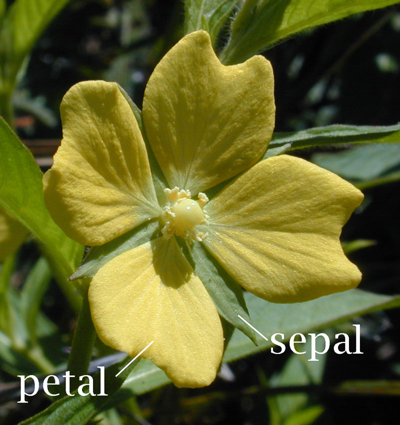
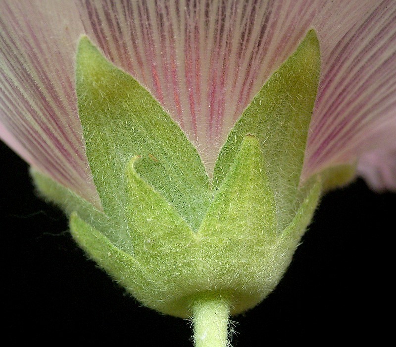
A sepal is the green leaf-like structure found underneath the petal in many flowers. Sepals provides protection for the flower when budding, and support for it once it is blooming.
Given that that is the case, we might expect plants with larger petals to also have larger sepals for additional support.
Can we predict the length of the petal of a plant from the length of its sepal?
import matplotlib.pyplot as plt

iris_dataset.plot("sepal_length", "petal_length", kind="scatter")
plt.show()

iris1 = iris_dataset.plot(
    "sepal_length",
    "petal_length",
    kind="scatter",
    title="Petal and sepal length in three species of Iris"
)
iris1.set_xlabel("Sepal length (cm)")
iris1.set_ylabel("Petal length (cm)")
plt.show()

Looks like the answer is... yes! If we draw a line across the plot, we can predict what the petal length might be for a plant given a particular sepal length.
That's all a model is! -- something that can extrapolate from known data to predict what the value might be for a given input value.
Linear regression can define that model precisely
Drawing a line by hand is fine, but we would like to determine exactly how the petal length varies as the sepal length varies. Luckily, matplotlib can run a linear regression for us easily.
iris_dataset.sepal_length.head()
0    5.1
1    4.9
2    4.7
3    4.6
4    5.0
Name: sepal_length, dtype: float64
iris_dataset.petal_length.head()
0    1.4
1    1.4
2    1.3
3    1.5
4    1.4
Name: petal_length, dtype: float64
Scikit-learn's LinearRegression module needs the data as a two-dimensional array:
- It expects each row to contain multiple features.
- It expects as many rows as there are data points.
iris_dataset.sepal_length.values.reshape(-1, 1)
array([[5.1],
       [4.9],
       [4.7],
       [4.6],
       [5. ],
       [5.4],
       [4.6],
       [5. ],
       [4.4],
       [4.9],
       [5.4],
       [4.8],
       [4.8],
       [4.3],
       [5.8],
       [5.7],
       [5.4],
       [5.1],
       [5.7],
       [5.1],
       [5.4],
       [5.1],
       [4.6],
       [5.1],
       [4.8],
       [5. ],
       [5. ],
       [5.2],
       [5.2],
       [4.7],
       [4.8],
       [5.4],
       [5.2],
       [5.5],
       [4.9],
       [5. ],
       [5.5],
       [4.9],
       [4.4],
       [5.1],
       [5. ],
       [4.5],
       [4.4],
       [5. ],
       [5.1],
       [4.8],
       [5.1],
       [4.6],
       [5.3],
       [5. ],
       [7. ],
       [6.4],
       [6.9],
       [5.5],
       [6.5],
       [5.7],
       [6.3],
       [4.9],
       [6.6],
       [5.2],
       [5. ],
       [5.9],
       [6. ],
       [6.1],
       [5.6],
       [6.7],
       [5.6],
       [5.8],
       [6.2],
       [5.6],
       [5.9],
       [6.1],
       [6.3],
       [6.1],
       [6.4],
       [6.6],
       [6.8],
       [6.7],
       [6. ],
       [5.7],
       [5.5],
       [5.5],
       [5.8],
       [6. ],
       [5.4],
       [6. ],
       [6.7],
       [6.3],
       [5.6],
       [5.5],
       [5.5],
       [6.1],
       [5.8],
       [5. ],
       [5.6],
       [5.7],
       [5.7],
       [6.2],
       [5.1],
       [5.7],
       [6.3],
       [5.8],
       [7.1],
       [6.3],
       [6.5],
       [7.6],
       [4.9],
       [7.3],
       [6.7],
       [7.2],
       [6.5],
       [6.4],
       [6.8],
       [5.7],
       [5.8],
       [6.4],
       [6.5],
       [7.7],
       [7.7],
       [6. ],
       [6.9],
       [5.6],
       [7.7],
       [6.3],
       [6.7],
       [7.2],
       [6.2],
       [6.1],
       [6.4],
       [7.2],
       [7.4],
       [7.9],
       [6.4],
       [6.3],
       [6.1],
       [7.7],
       [6.3],
       [6.4],
       [6. ],
       [6.9],
       [6.7],
       [6.9],
       [5.8],
       [6.8],
       [6.7],
       [6.7],
       [6.3],
       [6.5],
       [6.2],
       [5.9]])
from sklearn.linear_model import LinearRegression

X = iris_dataset.sepal_length.values.reshape(-1, 1)
Y = iris_dataset.petal_length

model = LinearRegression()
model.fit(X, Y)
slopes = model.coef_
intercept = model.intercept_

print(slopes, intercept)
[1.85750967] -7.0953814782793145
In other words, based on the available data, we can construct a model that predicts a petal length given a particular sepal length.
$$petal\_length = 1.8575 * sepal\_length - 7.095$$The Equation of a Line
You may be familiar with this as the equation of a line:
$$ y = mx + c $$See how easy it is to predict a petal value given a sepal value: you just plug it into the equation! For example:
# What is the predicted petal length when the sepal length is 5cm?
sepal_length = 5
petal_length = 1.8575 * sepal_length - 7.095
print(petal_length)
2.1925
# We could be more precise by plugging in the slope and intercept values directly.
petal_length = slopes[0] * sepal_length + intercept
print(petal_length)
2.192166848827913
Machine learning? For real?
Yes! By convention, we write this equation like this when thinking about it in machine-learning terms:
$$ y' = b + w_1x_1 $$Where:
- $y'$ is the predicted label (the desired output), which in our example is the petal length in centimeters.
- $b$ is the bias (the y-intercept, sometimes referred to as $w_0$), which in our example is 7.095 cm.
- $w_1$ is the weight of feature 1, which is the same concept as the "slope" in the traditional equation of the line. In our example, this is 1.8575.
- $x_1$ is a feature (a known input), which in our example is the sepal length.
Writing it in this way makes it easy to extend our model when we are considering multiple features, such as sepal length and sepal width and many more. In that case, our equation would look like:
$$ y' = b + w_1x_1 + w_2x_2 + w_3x_3 + \ldots + w_nx_n $$What does this model actually look like?
We can draw this model onto our plot from earlier as a line of best fit.
iris1 = iris_dataset.plot("sepal_length", "petal_length", kind="scatter", title="Petal and sepal length in three species of Iris", color="red")
iris1.set_xlabel("Sepal length (cm)")
iris1.set_ylabel("Petal length (cm)")

iris1.plot(iris_dataset.sepal_length, iris_dataset.sepal_length * slopes[0] + intercept, 'black')

plt.show()

Err...
You might have noticed that this is not a very good model:
- There's a lot of points at the bottom of the figure that don't follow the predicted relationship.
- Petal sizes above 3cm seem to be increasing less quickly as sepal size increases than the predicted relationship.
Let's calculate the predicted petal length for each flower -- what does our model predict as compared to the actual petal length we see?
data = pd.DataFrame({
    'sepal_length': iris_dataset.sepal_length,
    'petal_length': iris_dataset.petal_length
})
data['predicted_petal_length'] = data.sepal_length * slopes[0] + intercept
data.head()
| sepal_length | petal_length | predicted_petal_length | |
|---|---|---|---|
| 0 | 5.1 | 1.4 | 2.377918 |
| 1 | 4.9 | 1.4 | 2.006416 |
| 2 | 4.7 | 1.3 | 1.634914 |
| 3 | 4.6 | 1.5 | 1.449163 |
| 4 | 5.0 | 1.4 | 2.192167 |
If we plot the predicted petal length against the actual petal length, what would we expect to see?
predicted1 = data.plot('petal_length', 'predicted_petal_length', kind='scatter', color='red')
predicted1.plot(data.petal_length, data.petal_length, 'black')
plt.show()

Loss
Loss is a number indicating how bad the model's prediction was on one particular data point. If the model's prediction is perfect, the loss is zero; otherwise, the loss is greater. The goal of training a model is to find a set of weights and biases that have low loss, on average, across all examples.
In this example, we have 150 data points that provide a feature (the sepal length) as well as the label (the petal length). We can use these to determine how much total loss our model has over this dataset by calculating predicted labels and comparing them to the actual labels.
There are many different measures of loss. One common measure of loss that is particularly useful in linear regressions is squared loss (or $L_2$ loss). This is defined as the square of the difference between the label and the prediction. In other words, it is equal to: $$ = (predicted\ label - actual\ label)^2 $$ $$ = (observation - prediction(x))^2 $$ $$ = (y - y')^2 $$
We can use this equation to find the loss for a single data point. What does this look like in Python?
data['squared_error'] = (data.petal_length - data.predicted_petal_length)**2
data.head()
| sepal_length | petal_length | predicted_petal_length | squared_error | |
|---|---|---|---|---|
| 0 | 5.1 | 1.4 | 2.377918 | 0.956323 |
| 1 | 4.9 | 1.4 | 2.006416 | 0.367740 |
| 2 | 4.7 | 1.3 | 1.634914 | 0.112167 |
| 3 | 4.6 | 1.5 | 1.449163 | 0.002584 |
| 4 | 5.0 | 1.4 | 2.192167 | 0.627528 |
But how can we measure our total loss across all our 150 data points?
Mean Square Error (MSE)
The Mean Square Error (MSE) can be calculated as the arithmetic mean of all squared losses in a particular dataset $D$. We can calculate this as the total squared loss divided by the number of data points, i.e.:
$$ MSE = \frac{1}{N} \sum_{(x, y)\ \in\ D}{(y - y')^2} $$What does this look like in Python?
data.squared_error.mean()
0.7423201713947026
Tada!
We now have:
- A model that allows us to predict (or infer) the petal length from the sepal length within this dataset.
- A measure for determining how much the prediction varied from the actual label, i.e. its loss.
- A measure for determining how well the model performed on a particular dataset.
Exercises
Here are a few exercises to test your understanding of this material.
Exercise 1
In the Iris flower dataset, we looked at whether we could predict the petal length based on sepal length.
For this exercise, try using the sepal width to predict petal width, find the equation of the line of best fit, and plot that line on the same graph.
import pandas
import numpy
import matplotlib.pyplot as plt

# Import Iris dataset.
iris_dataset = # How can we load our dataset?

# Plot sepal widths against petal widths.
iris_dataset.plot(
  # How do we plot this dataset?
)
plt.show()
# Hmm, this is NOT looking good. Oh well, let's see how awful it is!
# Construct our model.
slope, intercept = # How do we calculate the slope (weight) and intercept (bias).
print(slope, intercept)
iris1 = iris_dataset.plot(
  # How do you plot a pretty graph?
)
iris1.set_xlabel("#TODO")
iris1.set_ylabel("#TODO")
iris1.plot(
  # How can you plot the line of best fit?
)
plt.show()
Exercise 2
For the model that predicts petal length from sepal length in Exercise 1, calculate the Mean Square Error (MSE).
# Calculate predicted petal widths.
iris_dataset['predicted_petal_width'] = # How?
iris_dataset['squared_error'] = # How??
print("The mean squared error is: ",
  # How???
)