Lecture 2: Basics for General Use (1.5 Hours)
ABSTRACT
In the previous two lectures we invested in getting our machines set up to help us maximize our programming utility. In Lecture 2 we start to delve into Python, where we will:
- use an interactive Python interface called a REPL (read-evaluate-print-loop) to evaluate Python code,
- learn about types, indexing, functions, and classes in Python,
- discuss the general differences between Python 2 and 3 as well as good coding style guides,
- setup a Python interface that consists of a notebook with code and documentation cells called Jupyter Notebook.
Introduction to the Python Language (45 Minutes)
Python, like many other interpreted languages, can be used in an interactive manner known as REPL (read-evaluate-print-loop). Though the name "REPL" might be new, this way of using Python is quite similar to how many other environments work, including languages as diverse as Lisp and MATLAB/Octave. Using the Python REPL will allow us to get a handle on the language without having to worry about writing self-contained programs right away.
In particular, we'll use an enhanced REPL for Python called IPython, as this comes with a lot of nice features for scientific computation (to wit, IPython was designed by a particle-physics grad student, Fernando Pérez). To start IPython, launch a command line session (either PowerShell or bash, depending on your operating system), and run the ipython command:
$ ipython
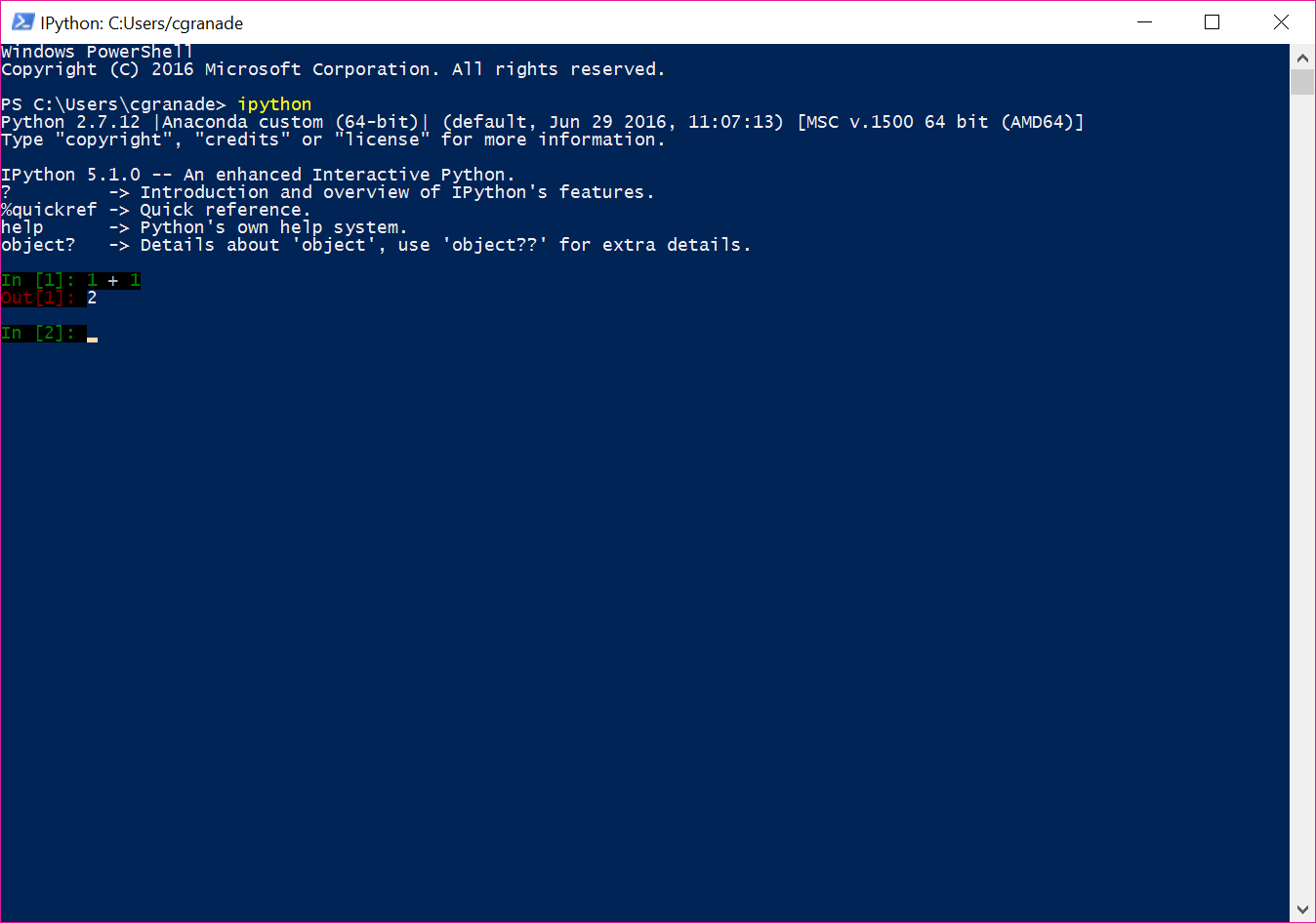
You'll be presented with a new shell that allows you to enter in Python expressions and statements. Let's try it out.
In [1]: 1 + 1
Out[1]: 2

In [2]:
Breaking this down a bit, 1 is a Python literal of type int (short for "integer") that we then add using the addition operator +. The expression 1 + 1 is then evaluated by IPython, and its value is printed out to the command line. We then loop to the next prompt, In [2]:.
NB: in a lot of Python documentation, you will often see >>> instead of numbered In prompts. The numbered prompts are an IPython feature, while >>> is the "plain" Python prompt. For the rest of this tutorial, I'll use the plain prompt for consistency with this convention.
Types in Python
Now that we see how to use IPython to run Python statements and expressions, let's use it to explore the language a bit more. First, let's familiarize ourselves with a few basic Python types and what we can do with them.
>>> x = "Hello, world!"
>>> print(x)
Hello, world!
In this example, "Hello, world!" is a string — that is, a sequence of characters representing text — that we can then display by using the function print(). Strings can be denoted using either single- or double-quotes, making it easy to nest strings. Triple quotes can be used to make multiline strings, but are otherwise identical.
>>> y = "What's up?"
>>> z = 'Just playing with \n some "quotes."'
>>> print(y + z)
What's up?Just playing with
 some "quotes."
>>> print("""foo
... bar""" == "foo\nbar")
True
In the above example, we also see two other important things about strings. First, that \n has a special meaning inside of a string, indicating a new line. This is an example of an escape character. Second, we note that the + operator acts differently for strings than for integers, and returns the concatenation of two strings. We will see more examples of how the behavior of operators such as + can depend on the type of its operands. For now, though, let's press on and see some other types that we can use.
One type that we will often rely on is bool, short for Boolean. This type is useful in that it only has two valid values, True and False, which are related by logical operators:
>>> True and True
True
>>> not True
False
>>> False or not True
False
Python also has a concept of things that are "truthy" and "falsy." This means that there are things (in this case other types) that the bool type will interpret as True and False. For example:
>>> bool('')
False
>>> bool([])
False
>>> bool(0)
False
>>> bool(0.00)
False
As you can see, anything that is "empty" or equivalent to 0 is interpreted as False. Things then that are "truthy" are then non-empty or non-zero:
>>> bool('abc')
True
>>> bool(['a',1,False])
True
>>> bool(-42)
True
>>> bool(3.14159)
True
Next, we will very often need to consider numbers other than integers. For this, the float type (short for "floating-point number") is very useful:
>>> float(1)
1.0
>>> 1 + 1.1
2.1
>>> 1 + 0.0
1.0
>>> 42.0 + float('inf')
inf
Here, we see that adding a float to an int results in a float, even if the float represents a number that is actually an integer. We also see that Python supports special non-numeric floating point values such as inf and nan (not a number) by using the float function with a string argument 'inf'. This demonstrates an important concept:
Python types are functions which return values of that type.
For instance:
>>> str()
''
>>> int()
0
>>> float()
0.0
>>> int("12")
12
We can use the type() function to return the type of a value:
>>> type(12)
<type 'int'>
Note that your output when using type() may differ from that presented here.
NB: the cheekier amongst us may wonder what the type of type is. For reasons that are both fascinating and esoteric, type(type) is type.
If you pass an argument to one of these type functions that cannot be interpreted, they function will raise an ValueError:
>>> float("foo")
Traceback (most recent call last):
  File "<stdin>", line 1, in <module>
ValueError: could not convert string to float: foo
>>> int("3.14159")
Traceback (most recent call last):
  File "<stdin>", line 1, in <module>
ValueError: invalid literal for int() with base 10: '3.14159'
Importantly, we can catch these errors and deal with them.
>>> try:
...     print(float("foo"))
... except ValueError:
...     print("nope.py")
...
nope.py
Python also supports several types for representing collections of different values. For instance, the list type does pretty much what it says on the tin:
>>> x = [12, 'foo', True]
>>> print(type(x))
<type 'list'>
Values of type list can be indexed by using the [] operator:
>>> print(x[0])
12
>>> print(x[2])
True
>>> print(type(x[2]))
<type 'bool'>
Note that Python starts indexing with zero. This is a very useful convention for programming, and will make our lives much, much simpler in a wide variety of ways. In particular, starting with 0 works very well in combination with slicing, where we index a list by a range instead of a single value. For instance:
>>> x = ['a', 'b', 'c', 'd']
>>> print(x[0:2])
['a', 'b']
>>> print(x[2:]) # If we omit the end of a slice, it continues until the end.
['c', 'd']
Python uses what are called half-open intervals to slice collections. We can think of this as indexing elements by "fence posts," as illustrated below.

When Python takes a slice of a list it returns all the objects "inside" the fences chosen by the slice. This example demonstrates that we can use slicing to partition a list without having to worry about adding and subtracting one, greatly reducing the opportunity for off-by-one errors. This benefit also extends to determining the lengths of collections:
>>> print(len(x))
4
>>> i = 1
>>> j = 3
>>> print(j - i == len(x[i:j]))
True
>>> assert(j - i == len(x[i:j]))
The len function above returns the length of a collection, allowing us to check that we the length of x[1:3] is the same as the distance between 1 and 3. We use the assert keyword, which raises an error if its argument is False, along with the equality operator == to check this.
Indexing also works over things other than lists:
>>> 'abcde'[1:3]
'bc'
>>> (1, 3.4, True, 'hi')[2:]
(True, 'hi')
In addition to list, Python also provides several other collection types. For instance, tuple is identical to list except that the contents of a tuple cannot be changed after it is created. That is, tuple values are immutable.
>>> x = [1, 2]
>>> x[1] = "foo"
>>> print(x)
[1, "foo"]
>>> x = (1, 2) # x is a tuple now!
>>> x[1] = 'bar'
Traceback (most recent call last):
  File "<ipython-input-21-3c6077352bf0>", line 1, in <module>
    x[1] = 'bar'
TypeError: 'tuple' object does not support item assignment
NB: as an annoying edge case, tuples with exactly one element must be written using a trailing comma, as in (2, ) to represent the tuple containing 2.
Also useful are dictionaries, also known as associative or mapping collections, represented in Python by the type dict. As opposed to indexing by consecutive integers, most immutable types (for instance, str, int, float and tuple) can be used to index a dictionary. Let's create a simple dictionary.
>>> x = {
...     'a': 'foo',
...     42: True,
...     (): 0.0
... }
>>> print(x[()])
0.0
>>> print(x['a'])
'foo'
NB: Note that the IPython REPL detected that the opening brace { of the dict was not closed, and changed the prompt to .... This indicates that the same line is being continued until a closing } is found. This will work for any type of character that the IPython REPL identifies as needing a closing or another line like [], {}, :, """, etc. Putting the dictionary entries on separate lines makes it easier to read.
Functions in Python
Now that we have an understanding of what basic types are available, we can move forward by writing some more useful code. Let's start by looking at how to define functions in Python.
>>> def f(x):
...     "Squares a thing"
...     return x ** 2 # ** is the exponentiation operator
...
>>> f(3)
9
The def keyword starts a function definition, and is followed by the name of the function and its arguments, followed by a colon. In the example above, we take one argument x. The body of a function is then set apart by indenting each line within the function. If the body of a function starts with a string, then that string becomes the function's documentation, known as its docstring. For f, we only have one actual line, return x ** 2, which squares the argument x and returns its value to the caller. Within IPython, function definitions require a final blank line, but this is not required outside of the REPL.
Functions can also take optional or keyword arguments, allowing arguments to have default values.
>>> def g(x, y, z=2):
...     return x + y ** z
...
>>> g(0, 2, 2)
4
>>> g(1, 2, 4)
17
>>> g(0, 2)
4
In addition, we can also pass arguments by name, useful for calling functions with a large number of arguments. That is to say, we can swap the order in which the arguments are listed as long as they are labeled as to which argument they are. If you label any of the arguments, you must label all remaining arguments to remove ambiguity.
>>> g(2, 3)
11
>>> g(y=3, z=2, x=5)
14
The issue of keyword arguments also gives us a good hint as to why some types in Python are immutable. In particular, immutability makes it much, much easier to eliminate some kinds of bugs. For instance, consider the following example:
>>> def sketchy_function(t=[]):
...     t.append("foo")
...     return t
...
>>> print(sketchy_function())
["foo"]
>>> print(sketchy_function())
["foo", "foo"]
So what is going wrong here? Because the default value for t is a mutable list then because the append method actually modifies the original list in-place. That is, the default value for t is still the same list, but that list now has different contents. This is most likely not the behavior desired for the function . Thankfully, there are better solutions that guarantee that t is initialized to [] by default every time the function is run without a value for t:
>>> def not_sketchy_function(t=None):
...     if t is None:
...         t = []
...     t.append("foo")
...     return t
...
>>> print(not_sketchy_function())
["foo"]
>>> print(not_sketchy_function())
["foo"]
Importantly, functions are values in and of themselves, and can be assigned to variables or passed as arguments.
>>> h = g
>>> h(3, 4)
81
>>> h
<function __main__.g>
Let's define a function that takes some other function and applies it twice.
>>> def apply_twice(f, x):
...     return f(f(x))
...
This is especially useful with lambda functions, which provide a way of defining one-line functions in a compact manner.
>>> (lambda x: x * 2 + '!')('ab')
'abab!'
>>> apply_twice((lambda x: x * 2 + '!'), 'ab')
'abab!abab!!'
We can use this to quickly apply a function over a collection, such as a list or a tuple, with the map function:
>>> list(map(lambda x: x ** 2 , [2, 3, 4]))
[4, 9, 16]
This example shows that map applies its first argument to each element of a collection. By calling list, we then make a new list to hold the results of map. We will discuss map a bit more later in this lecture.
Alternately, we can also use a list comprehension to represent the same idea in a way that more closely resembles "set builder notation."
>>> x = [2, 3, 4]
>>> y = [element ** 2 for element in x]
>>> print(y)
[4, 9, 16]
Underlying all of these examples is the concept of iteration, in which one value at a time is yielded from some collection. Functions such as list or map then iterate over their arguments, such that they can be used with any iterable value. Similarly, for loops consume iterators and act on each value at a time. For instance, list and tuple yield each of their elements, as we can see with a quick example.
>>> for element in [1, 'a', False]:
...     print(element)
...
1
'a'
False
This is a notable contrast to how for loops work in languages such as FORTRAN or C, and is most closely related to what many languages call a "for-each" loop. To emulate C- or FORTRAN-style for-loops, Python provides a function range that allows iterating over a collection of indices:
>>> for idx in range(3):
...     print(x[idx])
...
2
3
4
Iterators allow for writing writing for loops in a much more robust style, however, such that looping over range is not recommended. In particular, the enumerate function provides a very useful iterable. Let's look at a more complicated example, then break it down some:
>>> for idx, element in enumerate('abc'):
...     print("{} -- {}".format(idx, element))
...
0 -- a
1 -- b
2 -- c
As promised, let's look at each part of this example in turn. First, we now have two loop variables instead of one. This is an example of destructuring assignment, and works because each value yielded by enumerate is a tuple:
>>> print(list(enumerate('ab'))
[(0, 'a'), (1, 'b')]
Each of these tuples contains the index of an element and the element itself. Since str iterates and yields each character at a time, the "elements" are strings of length 1. In the for loop above, each of these tuples then gets "unpacked," such that idx is set to each index and element is set to each element.
Next, we see an example of format, which makes a new string from one or more other values. In the string "{} -- {}", each {} serves as a placeholder that is filled with the arguments to format:
>>> "{}, {}!".format('Hello', 'world')
'Hello, world!'
Python provides a rich set of tools for operating on iterable values, most notably through the built-in itertools package. We can include itertools by running the statement import itertools, as below.
>>> r = [2, 3, 4]
>>> import itertools as it
>>> print(list(it.product(r, [0, 1])))
[(2, 0), (2, 1), (3, 0), (3, 1), (4, 0), (4, 1)]
The import statement is an extremely useful one in general, and is the main way to include additional functionality into Python. For instance, if you have a file foo.py in your current directory, then import foo will run that file, saving all of its variables and functions into the new Python value foo, known as a module. Similarly, import can include functionality defined as packages, which are folders containing the specially-named file __init__.py, possibly along with other modules.
The import statement finds modules and packages by scanning a special variable sys.path. For example:
>>> import sys
>>> print(sys.path)
['', 'C:\\Anaconda3\\envs\\py27\\python27.zip', 'C:\\Anaconda3\\envs\\py27\\DLLs', 'C:\\Anaconda3\\envs\\py27\\lib', 'C:\\Anaconda3\\envs\\py27\\lib\\plat-win', 'C:\\Anaconda3\\envs\\py27\\lib\\lib-tk', 'C:\\Anaconda3\\envs\\py27', 'C:\\Anaconda3\\envs\\py27\\lib\\site-packages', ...]
Here, the empty string '' indicates the current directory, while the rest of the entries refer to the Python standard library, and to where utilities like pip and conda install additional packages. To install your own module or package to these locations, Python provides a very nice package called distutils you can look at, but this is out of scope for our current discussion.
In any case, import also allows you to give an alternate name to modules and packages that you import. In the example above, we gave the itertools package a short name it, and then referred to the product function included with itertools using it.product. This function iterates over tuples with one element drawn from each of its arguments. As such, it.product is not limited to integers.
>>> print(list(it.product('abc', 'xyz')))
[('a', 'x'), ('a', 'y'), ('a', 'z'), ('b', 'x'), ('b', 'y'), ('b', 'z'), ('c', 'x'), ('c', 'y'), ('c', 'z')]
Classes in Python
Finally, Python also allows us to define our own types, known as classes. A value whose type is a class is called an instance of that class. For example:
>>> class ExampleClass(object):
...     x = "some reasonable value"
...
>>> example_instance = ExampleClass()
>>> print(example_instance.x)
some reasonable value
>>> example_instance.x = 42
>>> print(example_instance.x)
42
In this example, object specifies that our new class should inherit from the class object that is built in to Python; we'll see more about this later. The assignment to x in the body of the class defines a new attribute of ExampleClass that we can obtain through the dot operator (.).
For now, though, we note that classes can specify behavior as well as data, in that functions can also be attributes of classes. A function defined in this way is called a method, and takes a special first argument called self that is always an instance of the class being defined. Let's make a new class and add a couple of methods this time.
>>> class D(object):
...     x = 'world'
...     b = 3
...     def say_hello(self):
...         print("Hello, {}!".format(self.x))
...
...     def do_math(self, a):
...         print("The sum of  {} + {} is {}".format(a, self.b, a + self.b))
...         self.b = a + self.b
...
>>> d = D()
>>> d.say_hello()
Hello, world!
We can see that when we call the say_hello method, we need not pass its self argument, as this is automatically set to the instance on which we're calling the method in the first place.
>>> d.do_math(4)
The sum of  4 + 3 is 7
>>> d.do_math(1)
The sum of  1 + 7 is 8
>>> d.b = 0
>>> d.do_math(5)
The sum of  5 + 0 is 5
Looking then at the do_math method, it takes one input (a), adds it to the stored value of the attribute b, and then set the new value of b to the sum. We can manually set the value of this attribute, and then this change is reflected when we try the do_math method after.
Magic and Help Commands
In addition to running Python code for us, IPython also supports a number of different commands called magic commands. These commands aren't valid Python, but represent instructions to the REPL environment. For instance, the %timeit magic command takes a bit of Python code and repeatedly runs it to estimate how long it takes. Let's see how long it takes to format a very long list into a string:
In [1]: %timeit "{}".format([0] * 100000)
100 loops, best of 3: 4.89 ms per loop
NB: we've switched back to IPython-style prompts to emphasize that magic commands do not* work in "plain" Python contexts.*
We'll see a few more magic commands as we go through the lectures, but there's a lot we won't have time to cover in full detail, and thus will mention only briefly:
%debug: Interactively debug a Python statement after it crashes.%prun: Run a Python statement while collecting full profiling data.%cd/%ls: Emulate the command line programs of the same names; useful for navigating without launching a new IPython session.
Perhaps the most useful IPython feature of all, though, is its help command feature. As a shortcut to viewing documentation, you can run a variable, class, module, or package name followed by a question mark as a command.
In [2]: str?
Docstring:
str(object='') -> string

Return a nice string representation of the object.
If the argument is a string, the return value is the same object.
Type:      type
Use two question marks (??) to get details about its implementation. Let's try it out with a small example.
In [3]: def f(x):
    ...:     """Does a thing."""
    ...:     return x ** 2
    ...:

In [4]: f??
Signature: f(x)
Source:
def f(x):
    """Does a thing."""
    return x ** 2
File:      c:\users\cgranade\<ipython-input-10-69a064096fa5>
Type:      function
Running Python Programs
Leaving the IPython REPL aside for a few moments, it's sometimes very useful to be able to write our own entire programs in Python that. Thankfully, the python command-line program lets us do that easily, so let's go on and try it out. Using your favorite text editor, make a new file called foo.py with the following contents:
import sys

if __name__ == "__main__":
    print("{} to world, hello!".format(sys.platform))
Use cd in the command line to navigate to the folder containing foo.py and run the following:
$ python foo.py
This works because when python runs a Python file, it sets the special variable __name__ to "__main__".
NB: the python command also takes a -m option (short for module), which finds a program to run using the same rules as import. For instance, python -m foo works in the above example, for the same reason that import foo would find foo.py.
A Few Words on Python 2 vs 3 (5 Minutes)
There are two different versions of Python, 2 and 3, that are in common use today. Python 3 brings with it a number of new features and clarifies a lot of earlier issues and edge cases, and is recommended for new projects. Though Python 2 is still being maintained for the foreseeable future, there are no new features that will be developed for the Python 2 language or standard library.
Unfortunately, moving to Python 3 is a bit more complicated for quantum information on Windows, as compiler support means that QuTiP is currently only stable on Windows with Python 2.7. For this reason, we strongly suggest writing code that is compatible with both versions 2 and 3, and will take a few moments to provide some tips to do so.
Most importantly to scientific computing, the definition of division has changed with Python 3 to be much more in line with what we might naively expect. On Python 2, 1 / 2 returns 0, as / between two integers is defined as returning an integer. In Python 3, 1 / 2 is automatically promoted to the floating-point value 0.5. If integer division is wanted, the // operator is available, such that 1 // 2 == 0 on Python 3.
The new behavior for / can be used even on Python 2.7 by using a special import statement at the top of each file:
from __future__ import division
The __future__ module allows for turning on forward-compatibility features, and is very handy in writing 2/3 compatible code. For instance, __future__ also provides the print_function feature to force print to be a function on Python 2; otherwise, print is defined as a keyword, and cannot be used in map or other contexts in which a function is expected.
The other important change to be aware of is that many Python 3 functions return iterators where their Python 2 counterparts returned lists. This change allows for lazy computation, in which a value isn't calculated until the iterator needs to yield it. As we saw above, list() allows for constructing lists explicitly from iterators, so that list(map(...)) will work on either 2 or 3. Similarly, range on Python 3 returns an iterator and returns a list on Python 2; though either works with a for loop, this means one should take some care before calling range with extremely large numbers.
For the most part, the split between 2 and 3 is an annoyance, but will not be a major problem for us if we take some proactive caution to write code that is compatible with both.
Style Guidelines for General Happiness (10 Minutes)
As with various English writing style guides to help people write with uniform grammar and formatting, there are coding style guides. The name of the Python guide is PEP 8. As with many style guide it is long to accommodate specifying lots of edge cases, but we'll look at some of the most common recommendations.
- Naming modules or Python files
Do not use a space in the file name! This will cause large problems when you try to import the file(s):
>>> import foo bar

  File "<ipython-input-5-3d3b554def9b>", line 1
    import foo bar
                 ^
SyntaxError: invalid syntax
>>> import foobar
- Spaces around binary operators:
When using operator symbols like +, -, =, +=, <, >, is, and, not, (and many more) there should be a space on each side of the operator.
total = a + b
val and not error == true
- Indents:
Always 4 spaces. Some text editors insert a special character called the tab character whenever you press the tab key (this is represented in Python by "\t"), which show up as any number of spaces. Python 2.x and older versions could understand a tab character mixed with spaces, but Python 3 and later require sticking with either spaces or tabs. If you don't like hitting the space bar 4 times, you can often configure your editor to auto convert between you hitting tab and entering 4 spaces (see earlier tutorial on setting up your editor).
NB: the Tab character really is a single character— try selecting the output in the cell below with your mouse! This isn't a great way in general to tell if something is a single character, after all emoji exist, but it demonstrates that something a bit funny is going on.
print("This is a tab: '\t'")
This is a tab: ' '
- Long expressions with binary operators
When an expression will not fit on one line, you should put the operator at the beginning of the line to make it easier to read:
total = (big_number1 + big_number2
    + big_number3
    - big_number4
    + big_number5)
- Naming things
- Never use 'l' (lowercase letter el), 'O' (uppercase letter oh), or 'I' (uppercase letter eye) as single letter variables, since they are hard to distinguish in some fonts.
- Class names should use CamelCase, as in
ExampleClass(). - Function names and variables should be lowercase, with words separated by underscores as necessary to improve readability, as in
long_function_name(). - Constants are should be all caps with underscores to separate words, as in
NUM_ITERATIONS. - If a variable name would conflict with a Python keyword (such as
classorlambda), add one trailing underscore, as inclass_to prevent syntax errors while still maintaining readability. - In the context of functions and variables inside of classes, there's a few other important conventions:
- Having one leading underscore (
_var_name) indicates an attribute is for "internal" use only, though it doesn't really hide it or enforce "privacy." - Two leading underscores mean the same as one, but also tell the Python interpreter to "hide" your new attribute.
- Having two leading and trailing underscores (
__var_name__) indicates the name of a special attribute, used by the Python interpreter itself. For instance,a.__add__(b)is called to resolvea + b. Do not use your own names of this form, but instead only use those defined in the Python documentation.
- Having one leading underscore (
Jupyter Notebook (30 Minutes)
Jupyter Notebooks (formerly IPython Notebooks) are really neat ways to share and run code that can be mixed with rich formatted documentation, notes, pictures, equations in LaTeX, etc. You might notice that what you are looking at currently is an example of such a notebook :) The idea is similar to Mathematica in that you have a document that consists of cells that can contain code from a variety of languages, which links to a kernel that can execute the code in the notebook. If you look in the top right corner of this page you can see what kernel is connected to the notebook (probably some version of Python).
We have already installed Jupyter since it comes with many scientific Python distributions like Anaconda. To use or make a notebook, we start by launching the Jupyter notebook app from the command line. This launches a kernel and links it to the notebook document, which is then displayed in your browser. Let's try this now. Open a new bash or Powershell terminal and navigate on your computer (as discussed in Lecture 0) to the cloned GitHub repository for this workshop.
$ jupyter notebook
This will automatically open a new browser tab, which should look something like this:

If for some reason the browser does not automatically launch you can open it yourself and just go to the address listed in the shell output. The address will looks like The Jupyter Notebook is running at: http://localhost:8888/ (it won't all ways be port 8888). You can then see all the files that were in the folder that you started Jupyter in and if you click on on a notebook file (.ipynb) it will open in a new tab, or if you want to start a new notebook you can in the top right click the new button and choose Python from under Notebooks.
Now that we have a notebook open, let's look at how to do cool stuff in it!
NB: all of the toolbar commands/navigation in the cells have keyboard shortcuts that you can find in the menu at the top under the help tab. Most of these consist of Ctrl+M* or Esc, followed by another letter.*
There are two main types of cell in the notebook, code cells and Markdown cells. Code cells execute code, just like the >>> Python REPL inputs we were using earlier. To do this, select a code cell, type what you would like to evaluate, and then run the cell by pushing Shift+Enter together.

For instance, we can use code cells to run a few of the examples from earlier in our new notebook:

When running Python cells, Jupyter Notebook uses IPython to communicate with your Python environment. Thus, Jupyter Notebook also supports many of the magic commands we saw above. In the code cell below, try out some of the Python commands we learned about above.
Markdown cells resemble code cells, except they do not have the In [ ]: prompt. With a cell selected (indicated by a box around the cell) you can change the type of cell by the dropdown menu in the toolbar (or by using the keyboard shortcut Ctrl+M, M):

Some things you can do in Markdown:
- Type in plaintext
- Use Markdown to
**Bold**Bold*italicise*italicize~~strikethrough~~strikethrough- and apply many other standard formatting styles (ex. the bullets in this cell)
- Type LaTeX in math mode:
$\int_{a}^{b} x^2 dx$$~~\rightarrow~~$ $\int_{a}^{b} x^2 dx$. - Have LaTeX in a separate line:
$$\sum_{n=1}^{\infty} 2^{-n} = 1$$$~~\rightarrow$ $$\sum_{n=1}^{\infty} 2^{-n} = 1.$$ - Insert pictures with HTML (this is the code for the picture above)
<figure style="text-align: center;">
        <img src="files/figures/jupyter-change-cell.png" width="60%">
        <caption>Changing they type of cell with the toolbar</caption>
    </figure>
Test some of these out in the Markdown cell below. First double-click the cell to begin editing. When you would like to see how it looks, press Shift+Enter to execute the Markdown.
NB: All of the formatting in these notes is done with Markdown cells in the Jupyter Notebook (we will get to this later). When writing documentation for your projects, readme files, or just notes to yourself, Markdown can be a powerful formatting tool as well. For all the things you can do with Markdown see here or here, and if you are using GitHub (or something that supports most of GitHub's additions to Markdown) there is a great tutorial here.
This is a Markdown cell
A final note about the Jupyter notebooks is how to shut them down. Closing the tab does not actually stop the Jupyter app or the associated kernel. To close the app, just close the shell where you launched Jupyter from, or press Ctrl+C to interrupt the Notebook server.