Interactive Data Graphics with Plotly
In this lecture, we'll use the Plotly library to construct engaging interactive graphics using a high-level interface. We already worked with Plotly when we created attractive geographic data visualizations. In this lecture, we'll use Plotly to build out the rest of our standard data visualization tools.
There are a number of plot types not shown here: check the Plotly Express overview for many other interesting and useful plot types.
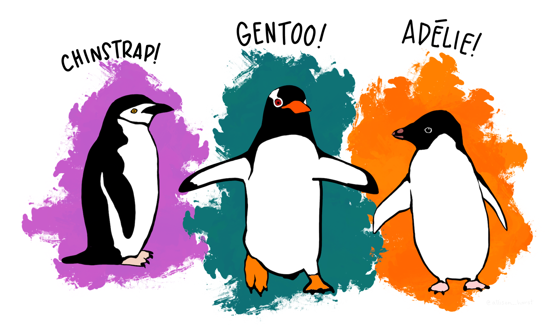
For this lecture, we're going to take a break from the NOAA climate data set. You'll use Plotly to construct visualizations using this data in HW1. For now, we're going to use the #BestDataSet: Palmer Penguins!
First, let's retrieve and clean up the data a little. These are all standard pandas operations, so we're not going to spend much time here.
import pandas as pd
url = "https://raw.githubusercontent.com/PhilChodrow/PIC16B/master/datasets/palmer_penguins.csv"
penguins = pd.read_csv(url)
penguins = penguins.dropna(subset = ["Body Mass (g)", "Sex"])
penguins["Species"] = penguins["Species"].str.split().str.get(0)
penguins = penguins[penguins["Sex"] != "."]

cols = ["Species", "Island", "Sex", "Culmen Length (mm)", "Culmen Depth (mm)", "Flipper Length (mm)", "Body Mass (g)"]
penguins = penguins[cols]
Let's take a look at the simplified data set:
penguins.head()
| Species | Island | Sex | Culmen Length (mm) | Culmen Depth (mm) | Flipper Length (mm) | Body Mass (g) | |
|---|---|---|---|---|---|---|---|
| 0 | Adelie | Torgersen | MALE | 39.1 | 18.7 | 181.0 | 3750.0 |
| 1 | Adelie | Torgersen | FEMALE | 39.5 | 17.4 | 186.0 | 3800.0 |
| 2 | Adelie | Torgersen | FEMALE | 40.3 | 18.0 | 195.0 | 3250.0 |
| 4 | Adelie | Torgersen | FEMALE | 36.7 | 19.3 | 193.0 | 3450.0 |
| 5 | Adelie | Torgersen | MALE | 39.3 | 20.6 | 190.0 | 3650.0 |
As you know from HW0, each row corresponds to an individual penguin. The penguin's species, island of encounter, and sex are recorded as qualitative variables. There are also measurements of the penguin's culmen (bill), as well as its flipper length and body mass. There are some additional columns which we're ignoring for today.
Getting Started with Plotly
Plotly includes a very large catalog of interesting plotting capabilities. We are only going to scratch the surface, using the Plotly Express module, which allows us to create several of the most important kinds of plots using convenient, high-level functions.
Let's run an example before breaking it down.
from plotly import express as px

fig = px.scatter(data_frame = penguins,
                 x = "Culmen Length (mm)",
                 y = "Culmen Depth (mm)",
                 color = "Species",
                 width = 500,
                 height = 300)

# reduce whitespace
fig.update_layout(margin={"r":0,"t":0,"l":0,"b":0})
# show the plot
fig.show()
Let's break this down a bit.
fig = px.scatter(data_frame = penguins,    # data set
                 x = "Culmen Length (mm)", # column for x axis
                 y = "Culmen Depth (mm)",  # column for y axis
                 color = "Species",        # column for dot color
                 width = 500,              # width of figure
                 height = 300)             # height of figure
Recall that our standard syntax from Matplotlib usually requires us to pass x and y as arrays or lists. Here, we do something different: we start by specifying a data frame. Then, x, y, and several other arguments that we'll see in a moment are interpreted as columns of the supplied data frame. So, a call like
fig = px.scatter(data_frame = penguins,
                 x = "Culmen Length (mm)",
                 y = "Culmen Depth (mm)")
is somewhat similar to
ax.scatter(penguins["Culmen Length (mm)"],
           penguins["Culmen Depth (mm)"])
using familiar Matplotlib tools. We'll see that the Plotly approach makes it much easier to construct complex data graphics in situations in which our data is in the form of a data frame.
Side note: the syntax of Plotly Express is similar to that of the Seaborn package, which is a non-interactive library for constructing complex graphics from data frames.
Let's fancy up our plot a little:
fig = px.scatter(data_frame = penguins,
                 x = "Culmen Length (mm)",
                 y = "Culmen Depth (mm)",
                 color = "Species",
                 hover_name = "Species",
                 hover_data = ["Island", "Sex"],
                 size = "Body Mass (g)",
                 size_max = 8,
                 width = 500,
                 height = 300,
                 opacity = 0.5)

# reduce whitespace
fig.update_layout(margin={"r":0,"t":0,"l":0,"b":0})
# show the plot
fig.show()
There are nice marginal plots for the statistically-inclined:
fig = px.scatter(data_frame = penguins,
                 x = "Culmen Length (mm)",
                 y = "Culmen Depth (mm)",
                 color = "Species",
                 hover_name = "Species",
                 hover_data = ["Island", "Sex"],
                 size = "Body Mass (g)",
                 size_max = 8,
                 width = 600,
                 height = 400,
                 opacity = 0.5,
                 marginal_y = "box",
                 marginal_x = "rug")

# reduce whitespace
fig.update_layout(margin={"r":0,"t":0,"l":0,"b":0})
# show the plot
fig.show()
Personally I dislike the gray background. It's possible to exercise fine-grained control over the plot appearance, but an easier way is through themes:
import plotly.io as pio

# for people who wish they were actually using R
# pio.templates.default = "ggplot2"

# my fave
pio.templates.default = "plotly_white"

# same plot as before
fig = px.scatter(data_frame = penguins,
                 x = "Culmen Length (mm)",
                 y = "Culmen Depth (mm)",
                 color = "Species",
                 hover_name = "Species",
                 hover_data = ["Island", "Sex"],
                 size = "Body Mass (g)",
                 size_max = 8,
                 width = 600,
                 height = 400,
                 opacity = 0.5,
                 marginal_y = "box",
                 marginal_x = "rug")

# reduce whitespace
fig.update_layout(margin={"r":0,"t":0,"l":0,"b":0})
# show the plot
fig.show()
Modifying the theme this way will change the appearance of all future plots.
Facets
Facetting refers to creating multiple, small plots, each of which display a subset of the data. Plotly supports the easy creation of facets using the facet_col and facet_row arguments.
fig = px.scatter(data_frame = penguins,
                 x = "Culmen Length (mm)",
                 y = "Culmen Depth (mm)",
                 color = "Species",
                 width = 600,
                 height = 300,
                 opacity = 0.5,
                 facet_col = "Sex")

# reduce whitespace
fig.update_layout(margin={"r":0,"t":50,"l":0,"b":0})
# show the plot
fig.show()
You can even use both at the same time!
fig = px.scatter(data_frame = penguins,
                 x = "Culmen Length (mm)",
                 y = "Culmen Depth (mm)",
                 color = "Species",
                 width = 600,
                 height = 300,
                 opacity = 0.5,
                 facet_col = "Island",
                 facet_row = "Sex")

# reduce whitespace
fig.update_layout(margin={"r":0,"t":50,"l":0,"b":0})
# show the plot
fig.show()
Faceting is an easy way to create complex, scientifically interesting plots using minimal effort.
fig = px.histogram(penguins,
                   x = "Culmen Length (mm)",
                   color = "Species",
                   opacity = 0.5,
                   nbins = 30,
                   barmode='stack',
                   width = 600,
                   height = 300)

# reduce whitespace
fig.update_layout(margin={"r":0,"t":0,"l":0,"b":0})
# show the plot
fig.show()
Boxplots
fig = px.box(penguins,
             x = "Species",
             y = "Body Mass (g)",
             color = "Sex",
             width = 600,
             height = 300)

# reduce whitespace
fig.update_layout(margin={"r":0,"t":0,"l":0,"b":0})
# show the plot
fig.show()
Bivariate Distributions
A density heatmap is just a bivariate histogram:
fig = px.density_heatmap(penguins,
                         x = "Body Mass (g)",
                         y = "Flipper Length (mm)",
                         facet_row = "Sex",
                         nbinsx = 25,
                         nbinsy = 25)

fig.update_layout(margin={"r":0,"t":0,"l":0,"b":0})
fig.show()
Density contours provide a nice alternative:
fig = px.density_contour(penguins,
                         x = "Body Mass (g)",
                         y = "Flipper Length (mm)",
                         facet_row = "Sex",
                         color = "Species")

fig.update_layout(margin={"r":50,"t":0,"l":0,"b":0})
fig.show()
fig = px.scatter_3d(penguins,
                    x = "Body Mass (g)",
                    y = "Culmen Length (mm)",
                    z = "Culmen Depth (mm)",
                    color = "Species",
                    opacity = 0.5)

fig.update_layout(margin={"r":0,"t":0,"l":0,"b":0})
fig.show()
Alluvial Diagrams
Alluvial diagrams can be used to compare tabulations of categorical variables.
colors = {"Adelie"    : "#2a9d8f",
          "Chinstrap" : "#e9c46a",
          "Gentoo"    : "#e76f51"}

color_hex = penguins["Species"].map(colors)
fig = px.parallel_categories(penguins,
                             dimensions = ["Species", "Island", "Sex"],
                             color = color_hex,
                             height = 300)

fig.update_layout(margin={"r":20,"t":0,"l":20,"b":0})
fig.show()
This diagram makes it clear that Gentoo penguins are only found on Biscoe Island, and Gentoos are only found on Dream Island, while the sexes of penguins are approximately balanced for each species on each island.
Parallel Coordinates
One can construct similar visualizations for quantitative variables. These are interesting and support quite entertaining filtering operations, but can also be somewhat challenging to give a clean "look."
spec_ids = penguins["Species"].map({"Adelie"    : 1,
                                    "Chinstrap" : 2,
                                    "Gentoo"    : 3})

fig = px.parallel_coordinates(penguins,
                              dimensions = ["Culmen Depth (mm)",
                                            "Culmen Length (mm)",
                                            "Flipper Length (mm)",
                                            "Body Mass (g)"],
                              color = spec_ids,
                              color_continuous_scale=px.colors.diverging.Tealrose,
                              color_continuous_midpoint=2,
                              height = 400)

fig.show()
After you've made your amazing plot, you can then save it as HTML and include it in your blog.
from plotly.io import write_html
write_html(fig, "my_fancy_plot.html")
Takeaways For Today
- Plotly Express makes it unreasonably easy to create attractive, sophisticated, and interactive data graphics.
- Amidst all these tools, it's important to choose the one that's right for the story you want to tell -- if your story is simple, use a simple visualization.
- Penguins are very good birds.