Advanced Data Manipulation
Over the next two weeks or so, we'll develop a range of skills for advanced data analysis in Python. We'll handle questions like:
- What if our data is split over multiple files?
- What if our data is in the wrong shape?
- What if our data is too big to conveniently fit in memory?
To approach these questions, we'll develop some more advanced skills with the familiar pandas library. We'll also introduce new tools for plotting, including spatial plots, and take a brief look at databases.
Case Study: Global Warming
Throughout our study, we'll focus on a single data set. This is the Global Historical Climatology Network data set, compiled by the National Centers for Environmental Information of the US National Oceanic and Atmospheric Administration. This data set contains an extraordinarily detailed record of surface temperatures at tens of thousands of atmospheric measurement stations across the globe. It is thus an ideal, publicly available data set for studying global warming. As you know, global warming is one of the most important issues of our time, primarily because it threatens the natural habitat of nature's most majestic creature:

An additional reason to be concerned about global warming is that rising temperatures reduce snowfall, a necessary prerequisite for videos of panda bears falling off of snowmen:

Takeaways for Today
Here's what I want you to take away from this lecture:
- Many data visualization problems can be solved by data manipulation.
pandasprovides a number of handy methods for combining and reshaping your data.- Pandas are very clumsy animals.
Data Source and Format
I accessed the data here, and then did a small amount of manipulation in order to save it as a set of CSV files. The files are hosted online at
https://raw.githubusercontent.com/PhilChodrow/PIC16B/master/datasets/noaa-ghcn/decades/
There is a file for each decade between 1901 and 2020. Today, we'll use only the file containing the most recent data, 2011-2020.
import pandas as pd

# advanced plotting tools for data frames
# basically a bunch of matplotlib shortcuts
import seaborn as sns

from matplotlib import pyplot as plt
import numpy as np
interval = "2011-2020"
url = f"https://raw.githubusercontent.com/PhilChodrow/PIC16B/master/datasets/noaa-ghcn/decades/{interval}.csv"
df = pd.read_csv(url)
df.head(5)
| ID | Year | VALUE1 | VALUE2 | VALUE3 | VALUE4 | VALUE5 | VALUE6 | VALUE7 | VALUE8 | VALUE9 | VALUE10 | VALUE11 | VALUE12 | |
|---|---|---|---|---|---|---|---|---|---|---|---|---|---|---|
| 0 | ACW00011604 | 2011 | -83.0 | -132.0 | 278.0 | 1040.0 | 1213.0 | 1663.0 | 1875.0 | 1723.0 | 1466.0 | 987.0 | 721.0 | 428.0 |
| 1 | ACW00011604 | 2012 | 121.0 | -98.0 | 592.0 | 646.0 | 1365.0 | 1426.0 | 1771.0 | 1748.0 | 1362.0 | 826.0 | 620.0 | -234.0 |
| 2 | ACW00011604 | 2013 | -104.0 | -93.0 | -48.0 | 595.0 | NaN | 1612.0 | 1855.0 | 1802.0 | 1359.0 | 1042.0 | 601.0 | NaN |
| 3 | AE000041196 | 2011 | 1950.0 | 2060.0 | 2280.0 | 2760.0 | 3240.0 | 3447.0 | 3580.0 | 3650.0 | 3316.0 | 2940.0 | 2390.0 | 1905.0 |
| 4 | AE000041196 | 2012 | 1837.0 | 1987.0 | NaN | NaN | NaN | NaN | NaN | NaN | NaN | NaN | NaN | NaN |
As provided, the data set contains the following columns:
ID: the ID number of the station. We can use this to figure out which country the station is in, as well as the spatial location of the station.Year: the year of the measurement.VALUE1-VALUE12: the temperature measurements themselves.VALUE1contains the temperature measurements for January,VALUE2for February, and so on.- The measurements are in hundredths of a degree, Celsius.
# measurement in February in very first row of DF
df["VALUE2"].iloc[0]

# temperature in degrees C is

df["VALUE2"].iloc[0] / 100
-1.32
We can now do things like plot the temperature in January for a selected station:
station_df = df[df["ID"] == "AEM00041194"]
sns.lineplot(data = station_df, x = "Year", y = "VALUE1")
<AxesSubplot:xlabel='Year', ylabel='VALUE1'>

At this station, the average temperature in January was typically between 20 and 22 degrees Celsius during the timeframe.
While it can be useful to have the temperate time series, there's a lot of information missing from this plot. For example, we're only plotting for a single month of the year, and we are also only showing the observations from a single weather station. In this lecture, our goal will be to construct the following plot:
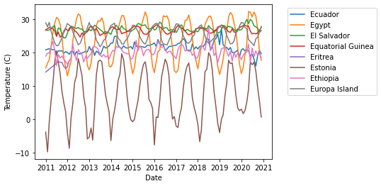
This is a plot of average temperatures over time for a selection of countries (ones whose names begin with E). In order to make this plot, there are two major data manipulation operations we need to perform. We need to:
- Figure out what country each station is in.
- Reshape the 12 month columns into a single long column.
These two tasks correspond to merging and stacking. These operations will come up at key points in our workflow.
Adding Countries with Merges
A merge is an operation that combines two related data frames into a single data frame, using one or more columns as keys. Let's take a look at how this works. The first thing we'll do is acquire a data frame that gives the full country name corresponding to the FIPS code. The FIPS code is an internationally standardized abbreviation for a country:
countries_url = "https://raw.githubusercontent.com/mysociety/gaze/master/data/fips-10-4-to-iso-country-codes.csv"
countries = pd.read_csv(countries_url)
countries.head(5)
| FIPS 10-4 | ISO 3166 | Name | |
|---|---|---|---|
| 0 | AF | AF | Afghanistan |
| 1 | AX | - | Akrotiri |
| 2 | AL | AL | Albania |
| 3 | AG | DZ | Algeria |
| 4 | AQ | AS | American Samoa |
How can we relate this to our df of temperature readings? Well, it turns out that the first two characters of the ID column give the FIPS code!
df["ID"].head(5)
0    ACW00011604
1    ACW00011604
2    ACW00011604
3    AE000041196
4    AE000041196
Name: ID, dtype: object
Let's extract them with the str attribute. Note that I am creating a new column whose name matches exactly the corresponding column in the countries data frame.
df["FIPS 10-4"] = df["ID"].str[0:2]
Now it's merge time. pandas provides a merge() function with many different arguments, as well as a related DataFrame.join() method. There are many different ways to merge two data sets, as explained in this helpful chapter of the Python Data Science Handbook. The default for pd.merge is an inner merge.
df = pd.merge(df, countries, on = ["FIPS 10-4"])
df.head(5)
| ID | Year | VALUE1 | VALUE2 | VALUE3 | VALUE4 | VALUE5 | VALUE6 | VALUE7 | VALUE8 | VALUE9 | VALUE10 | VALUE11 | VALUE12 | FIPS 10-4 | ISO 3166 | Name | |
|---|---|---|---|---|---|---|---|---|---|---|---|---|---|---|---|---|---|
| 0 | ACW00011604 | 2011 | -83.0 | -132.0 | 278.0 | 1040.0 | 1213.0 | 1663.0 | 1875.0 | 1723.0 | 1466.0 | 987.0 | 721.0 | 428.0 | AC | AG | Antigua and Barbuda |
| 1 | ACW00011604 | 2012 | 121.0 | -98.0 | 592.0 | 646.0 | 1365.0 | 1426.0 | 1771.0 | 1748.0 | 1362.0 | 826.0 | 620.0 | -234.0 | AC | AG | Antigua and Barbuda |
| 2 | ACW00011604 | 2013 | -104.0 | -93.0 | -48.0 | 595.0 | NaN | 1612.0 | 1855.0 | 1802.0 | 1359.0 | 1042.0 | 601.0 | NaN | AC | AG | Antigua and Barbuda |
| 3 | AE000041196 | 2011 | 1950.0 | 2060.0 | 2280.0 | 2760.0 | 3240.0 | 3447.0 | 3580.0 | 3650.0 | 3316.0 | 2940.0 | 2390.0 | 1905.0 | AE | AE | United Arab Emirates |
| 4 | AE000041196 | 2012 | 1837.0 | 1987.0 | NaN | NaN | NaN | NaN | NaN | NaN | NaN | NaN | NaN | NaN | AE | AE | United Arab Emirates |
What's happened here is the following:
- If the FIPS code in a row of
dfmatches a FIPS code incountries, then the corresponding columns ofcountriesare added to that row in themerged result. - If the FIPS code in a row of
dfis not found incountries, then that row is no longer present in themerged result.
Other behavior is possible. For example, one might instead prefer that, in case 2, the corresponding parts of the row are populated with NA values. This corresponds to a left join (rather than the default inner join).
We now have a few unnecessary columns, so we'll remove them.
df = df.drop(["FIPS 10-4", "ISO 3166"], axis = 1)
Stacking
Recall that we are aiming to create this figure:
We now know the country of each observation station, so that's good progress! But we have a bit of a problem now: we'd like to be able to plot all the months in the same time series in the logical way. We can't do this right now because each month's data is in a separate column. How can we create a single column containing the temperature observations?
The answer is that we can stack these columns into a single column. pandas provides a convenient method for stacking and unstacking data:
Here's how. First, we convert all the columns that we don't want to stack into a multi-index for the data frame.
df = df.set_index(keys=["ID", "Year", "Name"])
df.head()
| VALUE1 | VALUE2 | VALUE3 | VALUE4 | VALUE5 | VALUE6 | VALUE7 | VALUE8 | VALUE9 | VALUE10 | VALUE11 | VALUE12 | |||
|---|---|---|---|---|---|---|---|---|---|---|---|---|---|---|
| ID | Year | Name | ||||||||||||
| ACW00011604 | 2011 | Antigua and Barbuda | -83.0 | -132.0 | 278.0 | 1040.0 | 1213.0 | 1663.0 | 1875.0 | 1723.0 | 1466.0 | 987.0 | 721.0 | 428.0 |
| 2012 | Antigua and Barbuda | 121.0 | -98.0 | 592.0 | 646.0 | 1365.0 | 1426.0 | 1771.0 | 1748.0 | 1362.0 | 826.0 | 620.0 | -234.0 | |
| 2013 | Antigua and Barbuda | -104.0 | -93.0 | -48.0 | 595.0 | NaN | 1612.0 | 1855.0 | 1802.0 | 1359.0 | 1042.0 | 601.0 | NaN | |
| AE000041196 | 2011 | United Arab Emirates | 1950.0 | 2060.0 | 2280.0 | 2760.0 | 3240.0 | 3447.0 | 3580.0 | 3650.0 | 3316.0 | 2940.0 | 2390.0 | 1905.0 |
| 2012 | United Arab Emirates | 1837.0 | 1987.0 | NaN | NaN | NaN | NaN | NaN | NaN | NaN | NaN | NaN | NaN |
Then, we call the stack() method. This has the effect of "stacking" all of the data values on top of each other. There's also a new column indicating which of the original columns the observation came from:
df = df.stack()
df
ID           Year  Name
ACW00011604  2011  Antigua and Barbuda  VALUE1      -83.0
                                        VALUE2     -132.0
                                        VALUE3      278.0
                                        VALUE4     1040.0
                                        VALUE5     1213.0
                                                    ...
ZI000067983  2016  Zimbabwe             VALUE5     1692.0
                                        VALUE6     1681.0
                                        VALUE8     1828.0
                                        VALUE10    2334.0
                                        VALUE12    2287.0
Length: 1504990, dtype: float64
We can recover the ID, Year, and Name columns using reset_index():
df = df.reset_index()
df.head()
| ID | Year | Name | level_3 | 0 | |
|---|---|---|---|---|---|
| 0 | ACW00011604 | 2011 | Antigua and Barbuda | VALUE1 | -83.0 |
| 1 | ACW00011604 | 2011 | Antigua and Barbuda | VALUE2 | -132.0 |
| 2 | ACW00011604 | 2011 | Antigua and Barbuda | VALUE3 | 278.0 |
| 3 | ACW00011604 | 2011 | Antigua and Barbuda | VALUE4 | 1040.0 |
| 4 | ACW00011604 | 2011 | Antigua and Barbuda | VALUE5 | 1213.0 |
This is looking pretty good, except that the final two columns aren't labeled very appropriately. Let's fix that up:
df = df.rename(columns = {"level_3"  : "Month" , 0 : "Temperature (C)"})
df.head()
| ID | Year | Name | Month | Temperature (C) | |
|---|---|---|---|---|---|
| 0 | ACW00011604 | 2011 | Antigua and Barbuda | VALUE1 | -83.0 |
| 1 | ACW00011604 | 2011 | Antigua and Barbuda | VALUE2 | -132.0 |
| 2 | ACW00011604 | 2011 | Antigua and Barbuda | VALUE3 | 278.0 |
| 3 | ACW00011604 | 2011 | Antigua and Barbuda | VALUE4 | 1040.0 |
| 4 | ACW00011604 | 2011 | Antigua and Barbuda | VALUE5 | 1213.0 |
Better! We are now very close to our goal. The final step is to create a datetime column that reflects both the year and month. First, we can extract the month by picking out everything after the "VALUE" in the Month column.
df["Month"] = df["Month"].str[5:].astype(int)
df.head()
| ID | Year | Name | Month | Temperature (C) | |
|---|---|---|---|---|---|
| 0 | ACW00011604 | 2011 | Antigua and Barbuda | 1 | -83.0 |
| 1 | ACW00011604 | 2011 | Antigua and Barbuda | 2 | -132.0 |
| 2 | ACW00011604 | 2011 | Antigua and Barbuda | 3 | 278.0 |
| 3 | ACW00011604 | 2011 | Antigua and Barbuda | 4 | 1040.0 |
| 4 | ACW00011604 | 2011 | Antigua and Barbuda | 5 | 1213.0 |
Next, we'll create a new datetime column called Date. To do so, we can first create a string of the form YYYY-MM:
df["Date"] = df["Year"].astype(str) + "-" + df["Month"].astype(str)
df.head()
| ID | Year | Name | Month | Temperature (C) | Date | |
|---|---|---|---|---|---|---|
| 0 | ACW00011604 | 2011 | Antigua and Barbuda | 1 | -83.0 | 2011-1 |
| 1 | ACW00011604 | 2011 | Antigua and Barbuda | 2 | -132.0 | 2011-2 |
| 2 | ACW00011604 | 2011 | Antigua and Barbuda | 3 | 278.0 | 2011-3 |
| 3 | ACW00011604 | 2011 | Antigua and Barbuda | 4 | 1040.0 | 2011-4 |
| 4 | ACW00011604 | 2011 | Antigua and Barbuda | 5 | 1213.0 | 2011-5 |
We can convert the result to a DateTime using a built-in pandas function. The nice thing about this function is that it can automatically detect several common formats of date-time strings.
df["Date"] = pd.to_datetime(df["Date"])
df.head()
| ID | Year | Name | Month | Temperature (C) | Date | |
|---|---|---|---|---|---|---|
| 0 | ACW00011604 | 2011 | Antigua and Barbuda | 1 | -83.0 | 2011-01-01 |
| 1 | ACW00011604 | 2011 | Antigua and Barbuda | 2 | -132.0 | 2011-02-01 |
| 2 | ACW00011604 | 2011 | Antigua and Barbuda | 3 | 278.0 | 2011-03-01 |
| 3 | ACW00011604 | 2011 | Antigua and Barbuda | 4 | 1040.0 | 2011-04-01 |
| 4 | ACW00011604 | 2011 | Antigua and Barbuda | 5 | 1213.0 | 2011-05-01 |
Plotting
We are finally ready to make our plot! First, we compute the average temperature across all stations in each month, and divide by 100 to get units of degrees Celsius.
averages = df.groupby(["Name", "Date"])[["Temperature (C)"]].mean()/100
averages.head()
| Temperature (C) | ||
|---|---|---|
| Name | Date | |
| Afghanistan | 2011-01-01 | 5.136667 |
| 2011-02-01 | 6.280000 | |
| 2011-03-01 | 12.643333 | |
| 2011-04-01 | 19.070000 | |
| 2011-05-01 | 26.703333 |
Next, we'll turn the index columns into regular columns for plotting purposes.
averages = averages.reset_index()
averages.head()
| Name | Date | Temperature (C) | |
|---|---|---|---|
| 0 | Afghanistan | 2011-01-01 | 5.136667 |
| 1 | Afghanistan | 2011-02-01 | 6.280000 |
| 2 | Afghanistan | 2011-03-01 | 12.643333 |
| 3 | Afghanistan | 2011-04-01 | 19.070000 |
| 4 | Afghanistan | 2011-05-01 | 26.703333 |
Finally, we'll make the plot! To avoid overplotting, I'm going to plot only the countries whose English names begin with a given letter. The lineplot function of seaborn makes it easy to plot many labeled timeseries simultaneously.
begins_with = averages[averages["Name"].str[0] == "E"]

sns.lineplot(data = begins_with,
             x = "Date",
             y = "Temperature (C)",
             hue = "Name")

# legend needs to be adjusted
plt.legend(bbox_to_anchor=(1.05, 1),loc=2)
plt.savefig("pd-1-example-plot.png", bbox_inches = "tight")

We did it! Constructing this plot from the supplied data required us to merge and stack our data. This is a common pattern in applied data analysis -- we need to manipulate our data in a number of ways prior to the cool plotting or machine learning.
Takeaways for Today
Here's what I want you to take away from this lecture:
- Many data visualization problems can be solved by data manipulation.
pandasprovides a number of handy methods for combining and reshaping your data.- Pandas are very clumsy animals.