Mie Scattering of a Lossless Dielectric Sphere
A common reference calculation in computational electromagnetics for which an analytical solution is known is Mie scattering which involves computing the scattering efficiency of a single, homogeneous sphere given an incident planewave. The scattered power of any object (absorbing or non) can be computed by surrounding it with a closed DFT flux box (its size and orientation are irrelevant because of Poynting's theorem) and performing two simulations: (1) a normalization run involving an empty cell to save the incident fields from the source and (2) the scattering run with the object but first subtracting the incident fields in order to obtain just the scattered fields. This approach has already been described in Transmittance Spectrum of a Waveguide Bend.
The scattering cross section is the scattered power in all directions divided by the incident intensity. The scattering efficiency, a dimensionless quantity, is the ratio of the scattering cross section to the cross sectional area of the sphere. In this demonstration, the sphere is a lossless dielectric with wavelength-independent refractive index of 2.0. This way, subpixel smoothing can improve accuracy at low resolutions which is important for reducing the size of this 3d simulation. The source is an $E_z$-polarized, planewave pulse (its size parameter fills the entire cell in 2d) spanning the broadband wavelength spectrum of 10% to 50% the circumference of the sphere. There is one subtlety: since the planewave source extends into the PML which surrounds the cell on all sides, is_integrated=True must be specified in the source object definition. A k_point of zero specifying periodic boundary conditions is necessary in order for the source to be infinitely extended. Also, given the symmetry of the fields and the structure, two mirror symmery planes can be used to reduce the cell size by a factor of four. The simulation results are validated by comparing with the analytic theory obtained from the PyMieScatt module (which you will have to install in order to run the script below).
import meep as mp
import numpy as np
import matplotlib.pyplot as plt
import PyMieScatt as ps

r = 1.0  # radius of sphere

wvl_min = 2 * np.pi * r / 10
wvl_max = 2 * np.pi * r / 2

frq_min = 1 / wvl_max
frq_max = 1 / wvl_min
frq_cen = 0.5 * (frq_min + frq_max)
dfrq = frq_max - frq_min
nfrq = 100

## at least 8 pixels per smallest wavelength, i.e. np.floor(8/wvl_min)
resolution = 25

dpml = 0.5 * wvl_max
dair = 0.5 * wvl_max

pml_layers = [mp.PML(thickness=dpml)]

symmetries = [mp.Mirror(mp.Y), mp.Mirror(mp.Z, phase=-1)]

s = 2 * (dpml + dair + r)
cell_size = mp.Vector3(s, s, s)

# is_integrated=True necessary for any planewave source extending into PML
sources = [
    mp.Source(
        mp.GaussianSource(frq_cen, fwidth=dfrq, is_integrated=True),
        center=mp.Vector3(-0.5 * s + dpml),
        size=mp.Vector3(0, s, s),
        component=mp.Ez,
    )
]

sim = mp.Simulation(
    resolution=resolution,
    cell_size=cell_size,
    boundary_layers=pml_layers,
    sources=sources,
    k_point=mp.Vector3(),
    symmetries=symmetries,
)

box_x1 = sim.add_flux(
    frq_cen,
    dfrq,
    nfrq,
    mp.FluxRegion(center=mp.Vector3(x=-r), size=mp.Vector3(0, 2 * r, 2 * r)),
)
box_x2 = sim.add_flux(
    frq_cen,
    dfrq,
    nfrq,
    mp.FluxRegion(center=mp.Vector3(x=+r), size=mp.Vector3(0, 2 * r, 2 * r)),
)
box_y1 = sim.add_flux(
    frq_cen,
    dfrq,
    nfrq,
    mp.FluxRegion(center=mp.Vector3(y=-r), size=mp.Vector3(2 * r, 0, 2 * r)),
)
box_y2 = sim.add_flux(
    frq_cen,
    dfrq,
    nfrq,
    mp.FluxRegion(center=mp.Vector3(y=+r), size=mp.Vector3(2 * r, 0, 2 * r)),
)
box_z1 = sim.add_flux(
    frq_cen,
    dfrq,
    nfrq,
    mp.FluxRegion(center=mp.Vector3(z=-r), size=mp.Vector3(2 * r, 2 * r, 0)),
)
box_z2 = sim.add_flux(
    frq_cen,
    dfrq,
    nfrq,
    mp.FluxRegion(center=mp.Vector3(z=+r), size=mp.Vector3(2 * r, 2 * r, 0)),
)

sim.run(until_after_sources=10)

freqs = mp.get_flux_freqs(box_x1)
box_x1_data = sim.get_flux_data(box_x1)
box_x2_data = sim.get_flux_data(box_x2)
box_y1_data = sim.get_flux_data(box_y1)
box_y2_data = sim.get_flux_data(box_y2)
box_z1_data = sim.get_flux_data(box_z1)
box_z2_data = sim.get_flux_data(box_z2)

box_x1_flux0 = mp.get_fluxes(box_x1)

sim.reset_meep()

n_sphere = 2.0
geometry = [
    mp.Sphere(material=mp.Medium(index=n_sphere), center=mp.Vector3(), radius=r)
]

sim = mp.Simulation(
    resolution=resolution,
    cell_size=cell_size,
    boundary_layers=pml_layers,
    sources=sources,
    k_point=mp.Vector3(),
    symmetries=symmetries,
    geometry=geometry,
)

box_x1 = sim.add_flux(
    frq_cen,
    dfrq,
    nfrq,
    mp.FluxRegion(center=mp.Vector3(x=-r), size=mp.Vector3(0, 2 * r, 2 * r)),
)
box_x2 = sim.add_flux(
    frq_cen,
    dfrq,
    nfrq,
    mp.FluxRegion(center=mp.Vector3(x=+r), size=mp.Vector3(0, 2 * r, 2 * r)),
)
box_y1 = sim.add_flux(
    frq_cen,
    dfrq,
    nfrq,
    mp.FluxRegion(center=mp.Vector3(y=-r), size=mp.Vector3(2 * r, 0, 2 * r)),
)
box_y2 = sim.add_flux(
    frq_cen,
    dfrq,
    nfrq,
    mp.FluxRegion(center=mp.Vector3(y=+r), size=mp.Vector3(2 * r, 0, 2 * r)),
)
box_z1 = sim.add_flux(
    frq_cen,
    dfrq,
    nfrq,
    mp.FluxRegion(center=mp.Vector3(z=-r), size=mp.Vector3(2 * r, 2 * r, 0)),
)
box_z2 = sim.add_flux(
    frq_cen,
    dfrq,
    nfrq,
    mp.FluxRegion(center=mp.Vector3(z=+r), size=mp.Vector3(2 * r, 2 * r, 0)),
)

sim.load_minus_flux_data(box_x1, box_x1_data)
sim.load_minus_flux_data(box_x2, box_x2_data)
sim.load_minus_flux_data(box_y1, box_y1_data)
sim.load_minus_flux_data(box_y2, box_y2_data)
sim.load_minus_flux_data(box_z1, box_z1_data)
sim.load_minus_flux_data(box_z2, box_z2_data)

sim.run(until_after_sources=100)

box_x1_flux = mp.get_fluxes(box_x1)
box_x2_flux = mp.get_fluxes(box_x2)
box_y1_flux = mp.get_fluxes(box_y1)
box_y2_flux = mp.get_fluxes(box_y2)
box_z1_flux = mp.get_fluxes(box_z1)
box_z2_flux = mp.get_fluxes(box_z2)

scatt_flux = (
    np.asarray(box_x1_flux)
    - np.asarray(box_x2_flux)
    + np.asarray(box_y1_flux)
    - np.asarray(box_y2_flux)
    + np.asarray(box_z1_flux)
    - np.asarray(box_z2_flux)
)
intensity = np.asarray(box_x1_flux0) / (2 * r) ** 2
scatt_cross_section = np.divide(scatt_flux, intensity)
scatt_eff_meep = scatt_cross_section * -1 / (np.pi * r**2)
scatt_eff_theory = [
    ps.MieQ(n_sphere, 1000 / f, 2 * r * 1000, asDict=True)["Qsca"] for f in freqs
]
The incident intensity (intensity) is the flux in one of the six monitor planes (the one closest to and facing the planewave source propagating in the $x$ direction) divided by its area. This is why the six sides of the flux box are defined separately. (Otherwise, the entire box could have been defined as a single flux object with different weights ±1 for each side.) The scattered power is multiplied by -1 since it is the outgoing power (a positive quantity) rather than the incoming power as defined by the orientation of the flux box. Note that because of the linear $E_z$ polarization of the source, the flux through the $y$ and $z$ planes will not be the same. A circularly-polarized source would have produced equal flux in these two monitor planes. The runtime of the scattering run is chosen to be sufficiently long to ensure that the Fourier-transformed fields have converged.
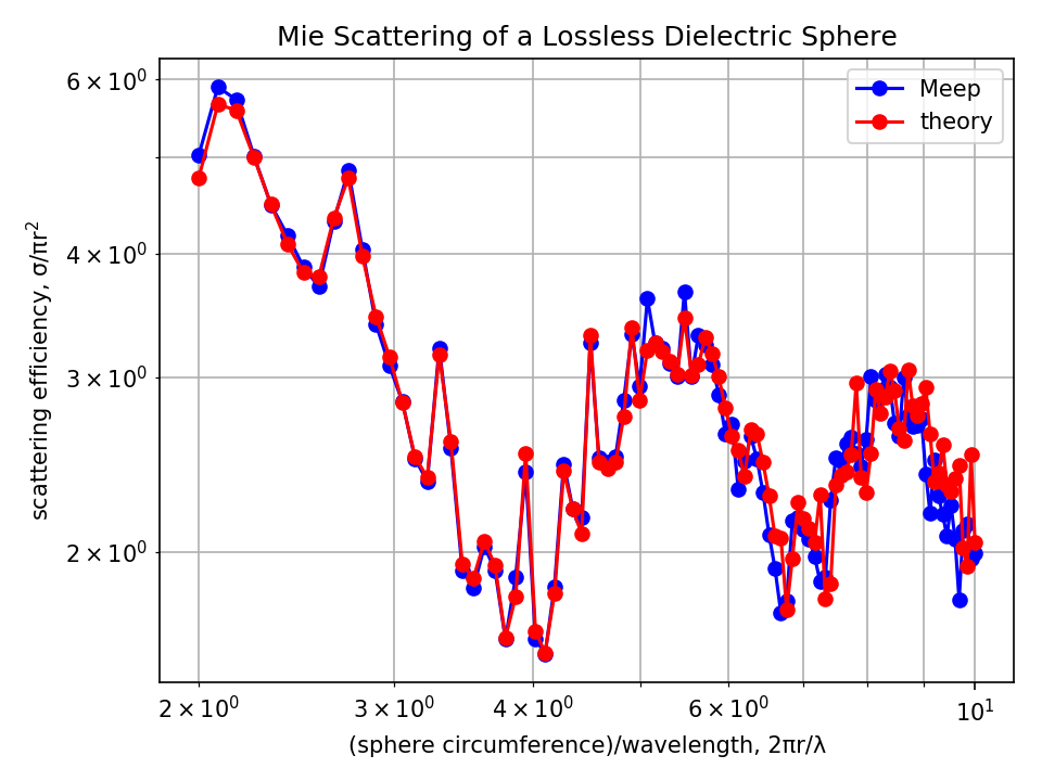
Results are shown below. Overall, the Meep results agree well with the analytic theory.
plt.figure(dpi=150)
plt.loglog(2 * np.pi * r * np.asarray(freqs), scatt_eff_meep, "bo-", label="Meep")
plt.loglog(2 * np.pi * r * np.asarray(freqs), scatt_eff_theory, "ro-", label="theory")
plt.grid(True, which="both", ls="-")
plt.xlabel("(sphere circumference)/wavelength, 2πr/λ")
plt.ylabel("scattering efficiency, σ/πr$^{2}$")
plt.legend(loc="upper right")
plt.title("Mie Scattering of a Lossless Dielectric Sphere")
plt.tight_layout()
plt.show()
Finally, for the case of a lossy dielectric material (i.e. complex refractive index) with non-zero absorption, the procedure to obtain the scattering efficiency is the same. The absorption efficiency is the ratio of the absorption cross section to the cross sectional area of the sphere. The absorption cross section is the total absorbed power divided by the incident intensity. The absorbed power is simply flux into the same box as for the scattered power, but without subtracting the incident field (and with the opposite sign, since absorption is flux into the box and scattering is flux out of the box): omit the load_minus_flux_data calls.