Download pre-trained models, in case you're in a hurry
#download pretrained models
!git clone https://github.com/Mainakdeb/deceptive-digits/
Cloning into 'deceptive-digits'...
remote: Enumerating objects: 125, done.
remote: Counting objects: 100% (125/125), done.
remote: Compressing objects: 100% (122/122), done.
remote: Total 125 (delta 40), reused 12 (delta 2), pack-reused 0
Receiving objects: 100% (125/125), 38.39 MiB | 27.69 MiB/s, done.
Resolving deltas: 100% (40/40), done.
Imports
import torch
import torchvision.transforms as transforms
import torchvision.utils as vutils
import torchvision.datasets as datasets
from torch.utils.data import DataLoader
import torch.nn as nn
import torch.optim as optim
import torch.nn.functional as F
from torch.autograd import Variable

import numpy as np
import matplotlib.pyplot as plt
import matplotlib.image as mimg
Misc:
device = torch.device("cuda" if torch.cuda.is_available() else "cpu")
workers = 2
batch_size = 64
image_size = 64
nc = 1 # Number of channels in the training images
nz = 100 # Size of z latent vector
ngf = 64 # Size of feature maps in generator
ndf = 64 # Size of feature maps in discriminator
lr = 2e-4 # Learning rate for optimizers
beta1 = 0.5 # eBta1 hyperparam for Adam optimizers
ngpu = 1

transforms = transforms.Compose(
    [
     transforms.Resize(image_size),
     transforms.RandomRotation(25),
     transforms.ToTensor(),
     transforms.Normalize(
         [0.5 for _ in range(nc)],
         [0.5 for _ in range(nc)]
         )
    ]
)

#dataset and dataloader
dataset = datasets.MNIST(root="/dataset/", train=True, transform=transforms, download=True)
dataloader = DataLoader(dataset, batch_size = batch_size, shuffle=True, drop_last=True)
Test if GPU is available
device
device(type='cuda')
Plot some samples from the trainloader
real_batch = next(iter(dataloader))
plt.figure(figsize=(8,8))
plt.axis("off")
plt.title("Training Images")
plt.imshow(np.transpose(vutils.make_grid(real_batch[0].to(device)[:64], padding=2, normalize=True).cpu(),(1,2,0)))
<matplotlib.image.AxesImage at 0x7f6ad6e5bed0>

The Generator network:
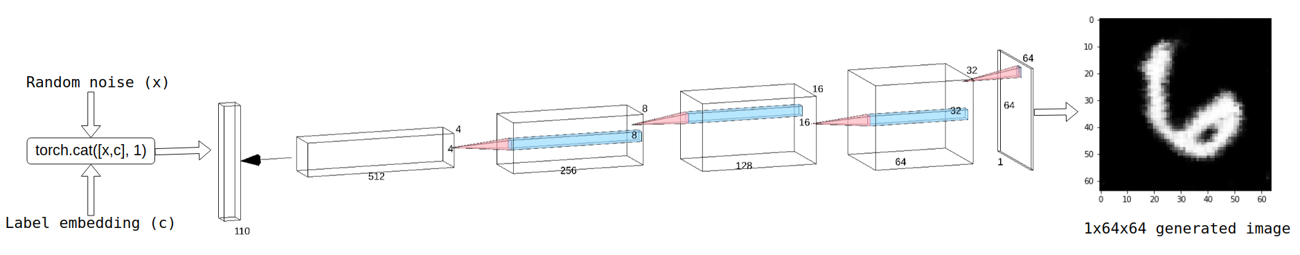
I concatenated a random noise vector of length 100 with another vector that represents a label of length 10 and passed the resulting tensor through the generator net. Notice that the input tensor has a length of 110. This input vector is passed through transpose-convolution layers to generate a 1x64x64 image.
class Generator(nn.Module):
    def __init__(self, params):
        super().__init__()

        self.label_emb = nn.Embedding(10, 10)

        self.tconv1 = nn.ConvTranspose2d(nz + 10, ngf * 8, kernel_size=4, stride=1, padding=0, bias=False)
        self.bn1 = nn.BatchNorm2d(ngf * 8)

        self.tconv2 = nn.ConvTranspose2d(ngf * 8, ngf * 4, 4, 2, 1, bias=False)
        self.bn2 = nn.BatchNorm2d(ngf * 4)

        self.tconv3 = nn.ConvTranspose2d(ngf * 4, ngf * 2, 4, 2, 1, bias=False)
        self.bn3 = nn.BatchNorm2d(ngf * 2)

        self.tconv4 = nn.ConvTranspose2d(ngf * 2, ngf, 4, 2, 1, bias=False)
        self.bn4 = nn.BatchNorm2d(ngf)

        self.tconv6 = nn.ConvTranspose2d(ngf, nc, 4, 2, 1, bias=False)

    def forward(self, x, labels):
        c = self.label_emb(labels)
        c = c.unsqueeze(2).unsqueeze(3)

        # print(c.size())
        # print(x.size())
        x = torch.cat([x, c], 1)
        x = F.relu(self.bn1(self.tconv1(x)))
        x = F.relu(self.bn2(self.tconv2(x)))
        x = F.relu(self.bn3(self.tconv3(x)))
        x = F.relu(self.bn4(self.tconv4(x)))
        # x = F.relu(self.bn5(self.tconv5(x)))
        x = torch.tanh(self.tconv6(x))

        return x


netG = Generator(ngpu).to(device)
print(netG)
Generator(
  (label_emb): Embedding(10, 10)
  (tconv1): ConvTranspose2d(110, 512, kernel_size=(4, 4), stride=(1, 1), bias=False)
  (bn1): BatchNorm2d(512, eps=1e-05, momentum=0.1, affine=True, track_running_stats=True)
  (tconv2): ConvTranspose2d(512, 256, kernel_size=(4, 4), stride=(2, 2), padding=(1, 1), bias=False)
  (bn2): BatchNorm2d(256, eps=1e-05, momentum=0.1, affine=True, track_running_stats=True)
  (tconv3): ConvTranspose2d(256, 128, kernel_size=(4, 4), stride=(2, 2), padding=(1, 1), bias=False)
  (bn3): BatchNorm2d(128, eps=1e-05, momentum=0.1, affine=True, track_running_stats=True)
  (tconv4): ConvTranspose2d(128, 64, kernel_size=(4, 4), stride=(2, 2), padding=(1, 1), bias=False)
  (bn4): BatchNorm2d(64, eps=1e-05, momentum=0.1, affine=True, track_running_stats=True)
  (tconv6): ConvTranspose2d(64, 1, kernel_size=(4, 4), stride=(2, 2), padding=(1, 1), bias=False)
)
The Discriminator network:
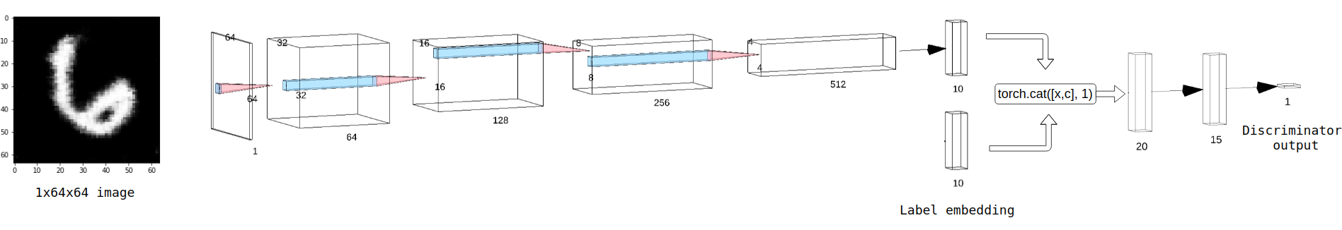
A 1x64x64 image is passed through convolution layers and the resulting tensor of length 10 is concatenated with a label embedding of length 10 and the resulting tensor is passed through the linear layers. Notice that the first linear layer takes an input of length 20. The final output is a tensor of length 1, which represents the probability of the sample being real or fake.
class Discriminator(nn.Module):
    def __init__(self, params):
        super().__init__()

        # meta data (label)
        self.label_emb = nn.Embedding(10, 10)

        self.conv1 = nn.Conv2d(nc, ndf, 4, 2, 1, bias=False)

        self.conv3 = nn.Conv2d(ndf, ndf * 2, 4, 2, 1, bias=False)
        self.bn3 = nn.BatchNorm2d(ndf * 2)

        self.conv4 = nn.Conv2d(ndf * 2, ndf * 4, 4, 2, 1, bias=False)
        self.bn4 = nn.BatchNorm2d(ndf * 4)

        self.conv5 = nn.Conv2d(ndf * 4, ndf * 8, 4, 2, 1, bias=False)
        self.bn5 = nn.BatchNorm2d(ndf * 8)

        self.conv6 = nn.Conv2d(ndf * 8, 10, 4, 1, 0, bias=False)

        self.fc1 = nn.Linear(20, 15)
        self.fc2 = nn.Linear(15, 1)

    def forward(self, x, labels):
        x = F.leaky_relu(self.conv1(x), 0.2, True)
        # print(x.size())
        # x = F.leaky_relu(self.bn2(self.conv2(x)), 0.2, True)
        # print(x.size())
        x = F.leaky_relu(self.bn3(self.conv3(x)), 0.2, True)
        x = F.leaky_relu(self.bn4(self.conv4(x)), 0.2, True)
        x = F.leaky_relu(self.bn5(self.conv5(x)), 0.2, True)
        x = F.leaky_relu(self.conv6(x))
        x = torch.flatten(x, 1)

        c = self.label_emb(labels)
        # print(x.size())
        # print(c.size())
        x = torch.cat([x, c], 1)
        # print(x.size())
        # print(c.size())
        x = F.leaky_relu(self.fc1(x))
        x = F.sigmoid(self.fc2(x))

        # print(x.size())

        return x


netD = Discriminator(ngpu).to(device)
print(netD)
Discriminator(
  (label_emb): Embedding(10, 10)
  (conv1): Conv2d(1, 64, kernel_size=(4, 4), stride=(2, 2), padding=(1, 1), bias=False)
  (conv3): Conv2d(64, 128, kernel_size=(4, 4), stride=(2, 2), padding=(1, 1), bias=False)
  (bn3): BatchNorm2d(128, eps=1e-05, momentum=0.1, affine=True, track_running_stats=True)
  (conv4): Conv2d(128, 256, kernel_size=(4, 4), stride=(2, 2), padding=(1, 1), bias=False)
  (bn4): BatchNorm2d(256, eps=1e-05, momentum=0.1, affine=True, track_running_stats=True)
  (conv5): Conv2d(256, 512, kernel_size=(4, 4), stride=(2, 2), padding=(1, 1), bias=False)
  (bn5): BatchNorm2d(512, eps=1e-05, momentum=0.1, affine=True, track_running_stats=True)
  (conv6): Conv2d(512, 10, kernel_size=(4, 4), stride=(1, 1), bias=False)
  (fc1): Linear(in_features=20, out_features=15, bias=True)
  (fc2): Linear(in_features=15, out_features=1, bias=True)
)
Initiate Weights
In the DCGAN paper, the authors specify that all model weights shall be randomly initialized from a Normal distribution with mean=0, stdev=0.02. The weights_init function takes an initialized model as input and reinitializes all convolutional, convolutional-transpose, and batch normalization layers to meet this criteria.
def weights_init(m):
    classname = m.__class__.__name__
    if classname.find('Conv') != -1:
        nn.init.normal_(m.weight.data, 0.0, 0.02)
    elif classname.find('BatchNorm') != -1:
        nn.init.normal_(m.weight.data, 1.0, 0.02)
        nn.init.constant_(m.bias.data, 0)

netD.apply(weights_init)
netG.apply(weights_init)
Generator(
  (label_emb): Embedding(10, 10)
  (tconv1): ConvTranspose2d(110, 512, kernel_size=(4, 4), stride=(1, 1), bias=False)
  (bn1): BatchNorm2d(512, eps=1e-05, momentum=0.1, affine=True, track_running_stats=True)
  (tconv2): ConvTranspose2d(512, 256, kernel_size=(4, 4), stride=(2, 2), padding=(1, 1), bias=False)
  (bn2): BatchNorm2d(256, eps=1e-05, momentum=0.1, affine=True, track_running_stats=True)
  (tconv3): ConvTranspose2d(256, 128, kernel_size=(4, 4), stride=(2, 2), padding=(1, 1), bias=False)
  (bn3): BatchNorm2d(128, eps=1e-05, momentum=0.1, affine=True, track_running_stats=True)
  (tconv4): ConvTranspose2d(128, 64, kernel_size=(4, 4), stride=(2, 2), padding=(1, 1), bias=False)
  (bn4): BatchNorm2d(64, eps=1e-05, momentum=0.1, affine=True, track_running_stats=True)
  (tconv6): ConvTranspose2d(64, 1, kernel_size=(4, 4), stride=(2, 2), padding=(1, 1), bias=False)
)
Load pretrained weights, in case you don't want to train.
# load
netG.load_state_dict(torch.load("/content/deceptive-digits/models/generator_w.pth"))
netD.load_state_dict(torch.load("/content/deceptive-digits/models/discriminator_w.pth"))
<All keys matched successfully>
fixed_noise = torch.randn(batch_size, nz, 1, 1, device=device)
real_label = 1.
fake_label = 0.

criterion = nn.BCELoss()
optimizerD = optim.Adam(netD.parameters(), lr=lr, betas=(beta1, 0.999))
optimizerG = optim.Adam(netG.parameters(), lr=lr, betas=(beta1, 0.999))

img_list = []
G_losses = []
D_losses = []
iters = 0
Training Loop
num_epochs = 6

for epoch in range(num_epochs):
    for i, data in enumerate(dataloader, 0):
        # (1) Update D network: maximize log(D(x)) + log(1 - D(G(z)))
        #print((data[1]))
        netD.zero_grad()
        # Format batch
        real_cpu = data[0].to(device)
        real_labels = data[1].to(device)
        b_size = real_cpu.size(0)
        label = torch.full((b_size,), real_label, dtype=torch.float, device=device)
        # Forward pass real batch through D
        output = netD(real_cpu, real_labels).view(-1)
        # Calculate loss on all-real batch
        # print(output[0])
        # print(label[0])
        errD_real = criterion(output, label)
        # Calculate gradients for D in backward pass
        errD_real.backward()
        D_x = output.mean().item()

        ## Train with all-fake batch
        # Generate batch of latent vectors
        noise = torch.randn(b_size, nz, 1, 1, device=device)
        fake_labels = Variable(torch.LongTensor(np.random.randint(0, 10, batch_size))).to(device)
        # Generate fake image batch with G
        fake = netG(noise, fake_labels)
        label.fill_(fake_label)
        # Classify all fake batch with D
        output = netD(fake.detach(), fake_labels).view(-1)
        # Calculate D's loss on the all-fake batch
        errD_fake = criterion(output, label)
        # Calculate the gradients for this batch
        errD_fake.backward()
        D_G_z1 = output.mean().item()
        # Add the gradients from the all-real and all-fake batches
        errD = errD_real + errD_fake
        # Update D
        optimizerD.step()

        ############################
        # (2) Update G network: maximize log(D(G(z)))
        ###########################
        netG.zero_grad()
        label.fill_(real_label)  # fake labels are real for generator cost
        # Since we just updated D, perform another forward pass of all-fake batch through D
        output = netD(fake, fake_labels).view(-1)
        # Calculate G's loss based on this output
        errG = criterion(output, label)
        # Calculate gradients for G
        errG.backward()
        D_G_z2 = output.mean().item()
        # Update G
        optimizerG.step()

        # print training stats
        if i % 50 == 0:
            print('[%d/%d][%d/%d]\tLoss_D: %.4f\tLoss_G: %.4f\tD(x): %.4f\tD(G(z)): %.4f / %.4f'
                  % (epoch, num_epochs, i, len(dataloader),
                     errD.item(), errG.item(), D_x, D_G_z1, D_G_z2))

        G_losses.append(errG.item())
        D_losses.append(errD.item())

        # Check how the generator is doing by saving G's output on fixed_noise
        if (iters % 500 == 0) or ((epoch == num_epochs-1) and (i == len(dataloader)-1)):
            with torch.no_grad():
                fake = netG(fixed_noise, fake_labels).detach().cpu()
            img_list.append(vutils.make_grid(fake, padding=2, normalize=True))

        iters += 1
[0/6][0/937] Loss_D: 1.3971 Loss_G: 0.8272 D(x): 0.4695 D(G(z)): 0.4724 / 0.4382
/usr/local/lib/python3.6/dist-packages/torch/nn/functional.py:1639: UserWarning: nn.functional.sigmoid is deprecated. Use torch.sigmoid instead.
  warnings.warn("nn.functional.sigmoid is deprecated. Use torch.sigmoid instead.")
/usr/local/lib/python3.6/dist-packages/torch/nn/functional.py:1628: UserWarning: nn.functional.tanh is deprecated. Use torch.tanh instead.
  warnings.warn("nn.functional.tanh is deprecated. Use torch.tanh instead.")
[0/6][50/937]	Loss_D: 0.0842	Loss_G: 4.3825	D(x): 0.9752	D(G(z)): 0.0569 / 0.0129
[0/6][100/937]	Loss_D: 0.2943	Loss_G: 4.7062	D(x): 0.9756	D(G(z)): 0.2324 / 0.0096
[0/6][150/937]	Loss_D: 0.3116	Loss_G: 3.8952	D(x): 0.9245	D(G(z)): 0.1988 / 0.0226
[0/6][200/937]	Loss_D: 0.7395	Loss_G: 3.4416	D(x): 0.8753	D(G(z)): 0.4216 / 0.0349
[0/6][250/937]	Loss_D: 0.2182	Loss_G: 2.9372	D(x): 0.9438	D(G(z)): 0.1449 / 0.0570
[0/6][300/937]	Loss_D: 0.4128	Loss_G: 2.7404	D(x): 0.8790	D(G(z)): 0.2350 / 0.0693
[0/6][350/937]	Loss_D: 2.2313	Loss_G: 3.4149	D(x): 0.1429	D(G(z)): 0.0099 / 0.0363
[0/6][400/937]	Loss_D: 4.1659	Loss_G: 0.0647	D(x): 0.9923	D(G(z)): 0.9831 / 0.9380
[0/6][450/937]	Loss_D: 0.6280	Loss_G: 3.0119	D(x): 0.8818	D(G(z)): 0.3645 / 0.0545
[0/6][500/937]	Loss_D: 0.9133	Loss_G: 1.4494	D(x): 0.6444	D(G(z)): 0.3306 / 0.2701
[0/6][550/937]	Loss_D: 0.8559	Loss_G: 1.5046	D(x): 0.6863	D(G(z)): 0.3354 / 0.2476
[0/6][600/937]	Loss_D: 0.6936	Loss_G: 3.5186	D(x): 0.9078	D(G(z)): 0.4189 / 0.0313
[0/6][650/937]	Loss_D: 0.8711	Loss_G: 2.0018	D(x): 0.8461	D(G(z)): 0.4568 / 0.1588
[0/6][700/937]	Loss_D: 1.0857	Loss_G: 2.5062	D(x): 0.8720	D(G(z)): 0.5794 / 0.0879
[0/6][750/937]	Loss_D: 0.9209	Loss_G: 1.3198	D(x): 0.4980	D(G(z)): 0.0986 / 0.3052
[0/6][800/937]	Loss_D: 0.5540	Loss_G: 1.5304	D(x): 0.7135	D(G(z)): 0.1686 / 0.2404
[0/6][850/937]	Loss_D: 0.7702	Loss_G: 1.0274	D(x): 0.6089	D(G(z)): 0.1568 / 0.3869
[0/6][900/937]	Loss_D: 0.5993	Loss_G: 2.4905	D(x): 0.7752	D(G(z)): 0.2608 / 0.0944
[1/6][0/937]	Loss_D: 0.7757	Loss_G: 1.3793	D(x): 0.6744	D(G(z)): 0.2614 / 0.2819
[1/6][50/937]	Loss_D: 0.7228	Loss_G: 1.4023	D(x): 0.6700	D(G(z)): 0.2307 / 0.2931
[1/6][100/937]	Loss_D: 0.9148	Loss_G: 2.2850	D(x): 0.8692	D(G(z)): 0.4818 / 0.1275
[1/6][150/937]	Loss_D: 0.5821	Loss_G: 1.8017	D(x): 0.7699	D(G(z)): 0.2365 / 0.1910
[1/6][200/937]	Loss_D: 0.6411	Loss_G: 2.5631	D(x): 0.8494	D(G(z)): 0.3406 / 0.0970
[1/6][250/937]	Loss_D: 0.7635	Loss_G: 1.5612	D(x): 0.6437	D(G(z)): 0.2274 / 0.2448
[1/6][300/937]	Loss_D: 0.8013	Loss_G: 1.5029	D(x): 0.5807	D(G(z)): 0.1512 / 0.2600
[1/6][350/937]	Loss_D: 0.9978	Loss_G: 2.7179	D(x): 0.9118	D(G(z)): 0.5325 / 0.0883
[1/6][400/937]	Loss_D: 0.8611	Loss_G: 1.2808	D(x): 0.5788	D(G(z)): 0.1938 / 0.3281
[1/6][450/937]	Loss_D: 0.6313	Loss_G: 1.9585	D(x): 0.7765	D(G(z)): 0.2858 / 0.1746
[1/6][500/937]	Loss_D: 0.7391	Loss_G: 2.4554	D(x): 0.7699	D(G(z)): 0.3353 / 0.1029
[1/6][550/937]	Loss_D: 0.9106	Loss_G: 1.9302	D(x): 0.7891	D(G(z)): 0.4410 / 0.1772
[1/6][600/937]	Loss_D: 0.6591	Loss_G: 2.1399	D(x): 0.7958	D(G(z)): 0.3036 / 0.1408
[1/6][650/937]	Loss_D: 0.7588	Loss_G: 2.7239	D(x): 0.8722	D(G(z)): 0.4266 / 0.0802
[1/6][700/937]	Loss_D: 0.6461	Loss_G: 2.1614	D(x): 0.8251	D(G(z)): 0.3364 / 0.1338
[1/6][750/937]	Loss_D: 0.8830	Loss_G: 2.7413	D(x): 0.9305	D(G(z)): 0.5074 / 0.0893
[1/6][800/937]	Loss_D: 0.6280	Loss_G: 1.9033	D(x): 0.7236	D(G(z)): 0.2164 / 0.1773
[1/6][850/937]	Loss_D: 0.6661	Loss_G: 1.9002	D(x): 0.6786	D(G(z)): 0.1895 / 0.1801
[1/6][900/937]	Loss_D: 0.6538	Loss_G: 2.6403	D(x): 0.8044	D(G(z)): 0.2855 / 0.0967
[2/6][0/937]	Loss_D: 0.5194	Loss_G: 1.9279	D(x): 0.7745	D(G(z)): 0.2098 / 0.1654
[2/6][50/937]	Loss_D: 0.5617	Loss_G: 1.9816	D(x): 0.7100	D(G(z)): 0.1482 / 0.1708
[2/6][100/937]	Loss_D: 0.3800	Loss_G: 2.8294	D(x): 0.8495	D(G(z)): 0.1699 / 0.0781
[2/6][150/937]	Loss_D: 0.6115	Loss_G: 1.9527	D(x): 0.7552	D(G(z)): 0.2306 / 0.1707
[2/6][200/937]	Loss_D: 0.5846	Loss_G: 1.9586	D(x): 0.7123	D(G(z)): 0.1596 / 0.1753
[2/6][250/937]	Loss_D: 0.4682	Loss_G: 2.1909	D(x): 0.7581	D(G(z)): 0.1341 / 0.1476
[2/6][300/937]	Loss_D: 0.6942	Loss_G: 2.1204	D(x): 0.7991	D(G(z)): 0.3167 / 0.1555
[2/6][350/937]	Loss_D: 0.5770	Loss_G: 2.1048	D(x): 0.7736	D(G(z)): 0.2133 / 0.1654
[2/6][400/937]	Loss_D: 0.4831	Loss_G: 2.8035	D(x): 0.8641	D(G(z)): 0.2354 / 0.0837
[2/6][450/937]	Loss_D: 0.5061	Loss_G: 1.8743	D(x): 0.7713	D(G(z)): 0.1754 / 0.1784
[2/6][500/937]	Loss_D: 0.6322	Loss_G: 2.3005	D(x): 0.7744	D(G(z)): 0.2387 / 0.1428
[2/6][550/937]	Loss_D: 0.6574	Loss_G: 2.2699	D(x): 0.7679	D(G(z)): 0.2409 / 0.1575
[2/6][600/937]	Loss_D: 0.6311	Loss_G: 2.7589	D(x): 0.7257	D(G(z)): 0.1886 / 0.0993
[2/6][650/937]	Loss_D: 0.6443	Loss_G: 2.1509	D(x): 0.8020	D(G(z)): 0.2779 / 0.1676
[2/6][700/937]	Loss_D: 0.6521	Loss_G: 2.6712	D(x): 0.8417	D(G(z)): 0.3076 / 0.1074
[2/6][750/937]	Loss_D: 0.6473	Loss_G: 2.1399	D(x): 0.8063	D(G(z)): 0.2996 / 0.1602
[2/6][800/937]	Loss_D: 0.8931	Loss_G: 1.3559	D(x): 0.5304	D(G(z)): 0.0916 / 0.3730
[2/6][850/937]	Loss_D: 0.6838	Loss_G: 2.6148	D(x): 0.7160	D(G(z)): 0.2071 / 0.1167
[2/6][900/937]	Loss_D: 0.9255	Loss_G: 1.2604	D(x): 0.5124	D(G(z)): 0.1315 / 0.3517
[3/6][0/937]	Loss_D: 0.7366	Loss_G: 2.1959	D(x): 0.7565	D(G(z)): 0.2887 / 0.1741
[3/6][50/937]	Loss_D: 1.0536	Loss_G: 3.2784	D(x): 0.9458	D(G(z)): 0.5445 / 0.0610
[3/6][100/937]	Loss_D: 0.7529	Loss_G: 1.6781	D(x): 0.6530	D(G(z)): 0.2017 / 0.2429
[3/6][150/937]	Loss_D: 1.0734	Loss_G: 1.2007	D(x): 0.4430	D(G(z)): 0.0949 / 0.3909
[3/6][200/937]	Loss_D: 0.7603	Loss_G: 1.6739	D(x): 0.6697	D(G(z)): 0.2230 / 0.2261
[3/6][250/937]	Loss_D: 0.7354	Loss_G: 1.4602	D(x): 0.6352	D(G(z)): 0.1611 / 0.3046
[3/6][300/937]	Loss_D: 1.3889	Loss_G: 1.7320	D(x): 0.6987	D(G(z)): 0.5518 / 0.2282
[3/6][350/937]	Loss_D: 0.9607	Loss_G: 1.1747	D(x): 0.5583	D(G(z)): 0.2123 / 0.3771
[3/6][400/937]	Loss_D: 0.7790	Loss_G: 2.2825	D(x): 0.7496	D(G(z)): 0.3221 / 0.1313
[3/6][450/937]	Loss_D: 0.8229	Loss_G: 1.6721	D(x): 0.7320	D(G(z)): 0.3311 / 0.2460
[3/6][500/937]	Loss_D: 0.8470	Loss_G: 1.4376	D(x): 0.5829	D(G(z)): 0.1670 / 0.2826
[3/6][550/937]	Loss_D: 0.5949	Loss_G: 1.7149	D(x): 0.7114	D(G(z)): 0.1652 / 0.2227
[3/6][600/937]	Loss_D: 1.1493	Loss_G: 3.6192	D(x): 0.9431	D(G(z)): 0.5955 / 0.0383
[3/6][650/937]	Loss_D: 1.4633	Loss_G: 1.1568	D(x): 0.7382	D(G(z)): 0.6039 / 0.3708
[3/6][700/937]	Loss_D: 0.7688	Loss_G: 1.5833	D(x): 0.7419	D(G(z)): 0.3252 / 0.2557
[3/6][750/937]	Loss_D: 0.8297	Loss_G: 1.6556	D(x): 0.7387	D(G(z)): 0.3431 / 0.2468
[3/6][800/937]	Loss_D: 1.1064	Loss_G: 1.9635	D(x): 0.7851	D(G(z)): 0.5087 / 0.1928
[3/6][850/937]	Loss_D: 0.9958	Loss_G: 1.7125	D(x): 0.7542	D(G(z)): 0.4460 / 0.2246
[3/6][900/937]	Loss_D: 0.8332	Loss_G: 1.5794	D(x): 0.6712	D(G(z)): 0.2693 / 0.2579
[4/6][0/937]	Loss_D: 0.7527	Loss_G: 2.5498	D(x): 0.6912	D(G(z)): 0.2502 / 0.1059
[4/6][50/937]	Loss_D: 1.0783	Loss_G: 1.9825	D(x): 0.7103	D(G(z)): 0.4452 / 0.1775
[4/6][100/937]	Loss_D: 1.3310	Loss_G: 0.7294	D(x): 0.3785	D(G(z)): 0.1405 / 0.5262
[4/6][150/937]	Loss_D: 0.8747	Loss_G: 2.3976	D(x): 0.8541	D(G(z)): 0.4427 / 0.1198
[4/6][200/937]	Loss_D: 0.7489	Loss_G: 1.4591	D(x): 0.6294	D(G(z)): 0.1773 / 0.2868
[4/6][250/937]	Loss_D: 0.9753	Loss_G: 1.8635	D(x): 0.7895	D(G(z)): 0.4552 / 0.2029
[4/6][300/937]	Loss_D: 1.0311	Loss_G: 1.8205	D(x): 0.5503	D(G(z)): 0.2423 / 0.2114
[4/6][350/937]	Loss_D: 1.0432	Loss_G: 0.9367	D(x): 0.5040	D(G(z)): 0.1967 / 0.4204
[4/6][400/937]	Loss_D: 1.4200	Loss_G: 2.3837	D(x): 0.8474	D(G(z)): 0.6336 / 0.1370
[4/6][450/937]	Loss_D: 0.9331	Loss_G: 1.5836	D(x): 0.6783	D(G(z)): 0.3480 / 0.2651
[4/6][500/937]	Loss_D: 1.0904	Loss_G: 1.8768	D(x): 0.6608	D(G(z)): 0.3935 / 0.2006
[4/6][550/937]	Loss_D: 1.1448	Loss_G: 1.3711	D(x): 0.5742	D(G(z)): 0.3842 / 0.2874
[4/6][600/937]	Loss_D: 1.3558	Loss_G: 3.0157	D(x): 0.7660	D(G(z)): 0.6017 / 0.0650
[4/6][650/937]	Loss_D: 1.2633	Loss_G: 2.1658	D(x): 0.7008	D(G(z)): 0.5326 / 0.1452
[4/6][700/937]	Loss_D: 1.2083	Loss_G: 1.9865	D(x): 0.6481	D(G(z)): 0.4676 / 0.1585
[4/6][750/937]	Loss_D: 1.1847	Loss_G: 1.3346	D(x): 0.5911	D(G(z)): 0.3854 / 0.3054
[4/6][800/937]	Loss_D: 1.4082	Loss_G: 2.1748	D(x): 0.7900	D(G(z)): 0.6284 / 0.1572
[4/6][850/937]	Loss_D: 1.1957	Loss_G: 1.3225	D(x): 0.6740	D(G(z)): 0.4614 / 0.3088
[4/6][900/937]	Loss_D: 1.1786	Loss_G: 1.8380	D(x): 0.7154	D(G(z)): 0.4976 / 0.1870
[5/6][0/937]	Loss_D: 1.1507	Loss_G: 1.4684	D(x): 0.6255	D(G(z)): 0.4345 / 0.2623
[5/6][50/937]	Loss_D: 1.0926	Loss_G: 1.2723	D(x): 0.5991	D(G(z)): 0.3765 / 0.3213
[5/6][100/937]	Loss_D: 1.0768	Loss_G: 1.5197	D(x): 0.7199	D(G(z)): 0.4753 / 0.2500
[5/6][150/937]	Loss_D: 1.1411	Loss_G: 1.2212	D(x): 0.5903	D(G(z)): 0.3983 / 0.3231
[5/6][200/937]	Loss_D: 1.1095	Loss_G: 1.2435	D(x): 0.5747	D(G(z)): 0.3661 / 0.3221
[5/6][250/937]	Loss_D: 1.9720	Loss_G: 3.9835	D(x): 0.8853	D(G(z)): 0.7631 / 0.0296
[5/6][300/937]	Loss_D: 1.0578	Loss_G: 1.7481	D(x): 0.6757	D(G(z)): 0.4372 / 0.2027
[5/6][350/937]	Loss_D: 0.7972	Loss_G: 1.4888	D(x): 0.6977	D(G(z)): 0.3161 / 0.2637
[5/6][400/937]	Loss_D: 0.8421	Loss_G: 2.0829	D(x): 0.7394	D(G(z)): 0.3842 / 0.1598
[5/6][450/937]	Loss_D: 2.5561	Loss_G: 0.3430	D(x): 0.1122	D(G(z)): 0.0759 / 0.7270
[5/6][500/937]	Loss_D: 1.0530	Loss_G: 1.2401	D(x): 0.5967	D(G(z)): 0.3583 / 0.3263
[5/6][550/937]	Loss_D: 1.2677	Loss_G: 1.0243	D(x): 0.5966	D(G(z)): 0.4830 / 0.3926
[5/6][600/937]	Loss_D: 1.4984	Loss_G: 0.9544	D(x): 0.3077	D(G(z)): 0.0869 / 0.4291
[5/6][650/937]	Loss_D: 0.9258	Loss_G: 1.5528	D(x): 0.6910	D(G(z)): 0.3851 / 0.2311
[5/6][700/937]	Loss_D: 0.6968	Loss_G: 3.2262	D(x): 0.8535	D(G(z)): 0.3587 / 0.0478
[5/6][750/937]	Loss_D: 1.1165	Loss_G: 1.5030	D(x): 0.6897	D(G(z)): 0.4750 / 0.2569
[5/6][800/937]	Loss_D: 0.8155	Loss_G: 2.5515	D(x): 0.8293	D(G(z)): 0.4170 / 0.1025
[5/6][850/937]	Loss_D: 0.8408	Loss_G: 4.6982	D(x): 0.8395	D(G(z)): 0.4356 / 0.0149
[5/6][900/937]	Loss_D: 0.8389	Loss_G: 1.5198	D(x): 0.6083	D(G(z)): 0.1918 / 0.2525
Visualize training metrics
plt.figure(figsize=(10,5))
plt.title("Generator and Discriminator Loss During Training")
plt.plot(G_losses,label="Gen")
plt.plot(D_losses,label="Disc")
plt.xlabel("iterations")
plt.ylabel("Loss")
plt.legend()
plt.show()

Generate one digit:
def generate_digit_from_label(label, seed):

  fake_label = torch.tensor([label]).cuda()
#   print("sn", single_noise.shape)
#   print("label", fake_label.shape)
  with torch.no_grad():
    fake_ = netG(seed, fake_label).detach().cpu()
#   print(single_noise.shape, fake_label.shape)
#   print(type(single_noise), type(fake_label))
  return(fake_.squeeze())


seed = torch.randn(1, nz, 1, 1, device=device)
plt.imshow(generate_digit_from_label(0, seed))
<matplotlib.image.AxesImage at 0x7f6ad21d27d0>

Generate images of all classes
fig, axes = plt.subplots(1,10, figsize = (20,8))

axes[0].set_title('label 0')
axes[0].imshow(generate_digit_from_label(0, seed), cmap="gray")
axes[1].set_title('label 1')
axes[1].imshow(generate_digit_from_label(1, seed), cmap="gray")
axes[2].set_title('label 2')
axes[2].imshow(generate_digit_from_label(2, seed), cmap="gray")
axes[3].set_title('label 3')
axes[3].imshow(generate_digit_from_label(3, seed), cmap="gray")
axes[4].set_title('label 4')
axes[4].imshow(generate_digit_from_label(4, seed), cmap="gray")
axes[5].set_title('label 5')
axes[5].imshow(generate_digit_from_label(5, seed), cmap="gray")
axes[6].set_title('label 6')
axes[6].imshow(generate_digit_from_label(6, seed), cmap="gray")
axes[7].set_title('label 7')
axes[7].imshow(generate_digit_from_label(7, seed), cmap="gray")
axes[8].set_title('label 8')
axes[8].imshow(generate_digit_from_label(8, seed), cmap="gray")
axes[9].set_title('label 9')
axes[9].imshow(generate_digit_from_label(9, seed), cmap="gray")
<matplotlib.image.AxesImage at 0x7f6ad1c5be50>

Exploring the Latent Space:
The generator net (here) accepts a latent vector of length 100 and a label embeddding of length 10. While the network trains, it learns to map these latent points to generated images. Every single latent vector is a point in an n-dimensional space where n is the length of the latent vector, which is 100 in this case.
What if you take 2 points in this 100-dimensional space and generate samples by interpolating between them? Every adjacent point leads to the generation of a slightly different image.
The folllowing cell generates images with latent vectors that are interpolated b/w 2 random points.
def generate_latent_points(latent_dim, n_samples, n_classes=10):
	# generate points in the latent space
	x_input = np.random.randn(latent_dim * n_samples)
	# reshape into a batch of inputs for the network
	z_input = x_input.reshape(n_samples, latent_dim)
	return z_input

# uniform interpolation between two points in latent space
def interpolate_points(p1, p2, n_steps=10):
	# interpolate ratios between the points
	ratios = np.linspace(0, 1, num=n_steps)
	# linear interpolate vectors
	vectors = list()
	for ratio in ratios:
		v = (1.0 - ratio) * p1 + ratio * p2
		vectors.append(v)
	return np.asarray(vectors)

n=20
pts = generate_latent_points(100, n)
interps = []
for i in range(0, n, 2):
    interpolated = interpolate_points(pts[i], pts[i+1], n_steps = 10)
    z = torch.tensor(interpolated).float().cuda()
    z=z.unsqueeze(2).unsqueeze(3)
    #print(z.shape)
    labels_ = torch.LongTensor(np.ones(10, dtype=int)*i//2).cuda()
    #print(labels_.shape)
    images = netG(z,labels_).detach().cpu().numpy()
    # for x in images:
    #     plt.imshow(x[0])
    #     plt.show()
    interps.append(images)
interps=np.array(interps)
Visualize images with neighbouring latent points
Notice how each frame is slightly different from the previous. Lets visualize some interpolations side by side, with a different set of interpolated points:
#Big Plot
fig, axes = plt.subplots(10,10, figsize = (20,20))
for i in range(0, 10):
    for j in range(0,10):
        axes[i,j].set_title('label '+str(i))
        axes[i,j].imshow(interps[i][j][0], cmap='gray')

plt.tight_layout()
plt.show()

The following gif showcases generated images with latent vectors interpolated between 2 points, looping back and forth between the 2 extremes.

Save interpolated images
The following cell was used to save frames, using which the above shown gif was made.
#save interpolations
fig, axes = plt.subplots(1,10, figsize = (70,10))
for j in range(0,10):
    for i in range(0, 10):
        axes[i].set_title('label '+str(i), FONTSIZE='3')
        axes[i].imshow(interps[i][j][0], cmap="gray")
        fig.savefig("interpolation_"+str(j)+".png") #create gif

for i in range(0,10):
    im = plt.imread("interpolation_"+str(i)+".png")
    plt.imshow(im)
    plt.show()
How Far Can We Go?
what if you wanted to generate images of numbers with multiple digits? I've used numpy to crop, invert and stich generated images horizontally, check out the generated image below.
def generate_and_save_image_with_multiple_digits(digits, seed):
  gen_list=[]
  for dig in str(digits):
    gen_list.append(generate_digit_from_label(int(dig), seed)[4:60, 10:58])
  vis = np.concatenate((gen_list), axis=1)
  vis = 255-vis
  mimg.imsave("generated"+str(digits)+".png", vis, cmap='gray')
  return(vis)
plt.imshow(generate_and_save_image_with_multiple_digits(12110, seed), cmap='gray')
plt.axis("off")
plt.show()
plt.imshow(generate_and_save_image_with_multiple_digits(410, seed), cmap='gray')
plt.axis("off")
plt.show()
plt.imshow(generate_and_save_image_with_multiple_digits(6789, seed), cmap='gray')
plt.axis("off")
plt.show()


So, can I make the model write phone numbers for me?
The results speak for themselves.
d=9830976450
plt.imshow(generate_and_save_image_with_multiple_digits(d, seed), cmap='gray')
plt.title("input: "+str(d))
plt.show()

Save model weights:
torch.save(netG.state_dict(), "generator_w.pth")
torch.save(netD.state_dict(), "discriminator_w.pth")