Notebook

Performing a convergence study¶

This example shows how to perform a convergence study to find an appropriate discretisation parameters for the Brillouin zone (kgrid) and kinetic energy cutoff (Ecut), such that the simulation results are converged to a desired accuracy tolerance.

Such a convergence study is generally performed by starting with a reasonable base line value for kgrid and Ecut and then increasing these parameters (i.e. using finer discretisations) until a desired property (such as the energy) changes less than the tolerance.

This procedure must be performed for each discretisation parameter. Beyond the Ecut and the kgrid also convergence in the smearing temperature or other numerical parameters should be checked. For simplicity we will neglect this aspect in this example and concentrate on Ecut and kgrid. Moreover we will restrict ourselves to using the same number of $k$ -points in each dimension of the Brillouin zone.

As the objective of this study we consider bulk platinum. For running the SCF conveniently we define a function:

In [1]:

using DFTK
using LinearAlgebra
using Statistics
using PseudoPotentialData

function run_scf(; a=5.0, Ecut, nkpt, tol)
    pseudopotentials = PseudoFamily("cp2k.nc.sr.lda.v0_1.largecore.gth")
    atoms    = [ElementPsp(:Pt, pseudopotentials)]
    position = [zeros(3)]
    lattice  = a * Matrix(I, 3, 3)

    model  = model_DFT(lattice, atoms, position;
                       functionals=LDA(), temperature=1e-2)
    basis  = PlaneWaveBasis(model; Ecut, kgrid=(nkpt, nkpt, nkpt))
    println("nkpt = $nkpt Ecut = $Ecut")
    self_consistent_field(basis; is_converged=ScfConvergenceEnergy(tol))
end;

Moreover we define some parameters. To make the calculations run fast for the automatic generation of this documentation we target only a convergence to 1e-2. In practice smaller tolerances (and thus larger upper bounds for nkpts and Ecuts are likely needed.

In [2]:

tol   = 1e-2      # Tolerance to which we target to converge
nkpts = 1:7       # K-point range checked for convergence
Ecuts = 10:2:24;  # Energy cutoff range checked for convergence

As the first step we converge in the number of $k$ -points employed in each dimension of the Brillouin zone …

In [3]:

function converge_kgrid(nkpts; Ecut, tol)
    energies = [run_scf(; nkpt, tol=tol/10, Ecut).energies.total for nkpt in nkpts]
    errors = abs.(energies[1:end-1] .- energies[end])
    iconv = findfirst(errors .< tol)
    (; nkpts=nkpts[1:end-1], errors, nkpt_conv=nkpts[iconv])
end
result = converge_kgrid(nkpts; Ecut=mean(Ecuts), tol)
nkpt_conv = result.nkpt_conv

nkpt = 1 Ecut = 17.0
n     Energy            log10(ΔE)   log10(Δρ)   Diag   Δtime
---   ---------------   ---------   ---------   ----   ------
  1   -26.49622281284                   -0.22    8.0    110ms
  2   -26.59233656940       -1.02       -0.63    2.0    158ms
  3   -26.61290867394       -1.69       -1.41    2.0   33.9ms
  4   -26.61326615223       -3.45       -2.13    2.0   31.5ms
nkpt = 2 Ecut = 17.0
n     Energy            log10(ΔE)   log10(Δρ)   Diag   Δtime
---   ---------------   ---------   ---------   ----   ------
  1   -25.79261308699                   -0.09    5.2   86.2ms
  2   -26.23307917121       -0.36       -0.70    2.0   56.2ms
  3   -26.23823144216       -2.29       -1.32    2.0   68.0ms
  4   -26.23848096839       -3.60       -2.32    1.0   48.0ms
nkpt = 3 Ecut = 17.0
n     Energy            log10(ΔE)   log10(Δρ)   Diag   Δtime
---   ---------------   ---------   ---------   ----   ------
  1   -25.78404837737                   -0.09    5.0   79.2ms
  2   -26.24025048195       -0.34       -0.80    2.0   57.1ms
  3   -26.25080534270       -1.98       -1.65    2.2   61.3ms
  4   -26.25104937780       -3.61       -2.22    1.0   46.1ms
nkpt = 4 Ecut = 17.0
n     Energy            log10(ΔE)   log10(Δρ)   Diag   Δtime
---   ---------------   ---------   ---------   ----   ------
  1   -25.91216018156                   -0.11    5.2    186ms
  2   -26.29428038427       -0.42       -0.77    2.0    116ms
  3   -26.30833081937       -1.85       -1.74    2.2    147ms
  4   -26.30842515507       -4.03       -2.66    1.0   91.4ms
nkpt = 5 Ecut = 17.0
n     Energy            log10(ΔE)   log10(Δρ)   Diag   Δtime
---   ---------------   ---------   ---------   ----   ------
  1   -25.90303612261                   -0.11    4.0    154ms
  2   -26.26717129897       -0.44       -0.72    2.0    115ms
  3   -26.28543617491       -1.74       -1.64    2.1    156ms
  4   -26.28571178256       -3.56       -2.28    1.0    346ms
nkpt = 6 Ecut = 17.0
n     Energy            log10(ΔE)   log10(Δρ)   Diag   Δtime
---   ---------------   ---------   ---------   ----   ------
  1   -25.87574090843                   -0.10    5.0    319ms
  2   -26.27389455410       -0.40       -0.77    1.9    208ms
  3   -26.28808182713       -1.85       -1.71    2.2    228ms
  4   -26.28818803673       -3.97       -2.62    1.0    162ms
nkpt = 7 Ecut = 17.0
n     Energy            log10(ΔE)   log10(Δρ)   Diag   Δtime
---   ---------------   ---------   ---------   ----   ------
  1   -25.89625074297                   -0.11    3.5    249ms
  2   -26.27883476796       -0.42       -0.75    2.0    187ms
  3   -26.29413133618       -1.82       -1.74    2.1    206ms
  4   -26.29420603226       -4.13       -2.65    1.0    145ms

Out[3]:

… and plot the obtained convergence:

In [4]:

using Plots
plot(result.nkpts, result.errors, dpi=300, lw=3, m=:o, yaxis=:log,
     xlabel="k-grid", ylabel="energy absolute error")

Out[4]:

We continue to do the convergence in Ecut using the suggested $k$ -point grid.

In [5]:

function converge_Ecut(Ecuts; nkpt, tol)
    energies = [run_scf(; nkpt, tol=tol/100, Ecut).energies.total for Ecut in Ecuts]
    errors = abs.(energies[1:end-1] .- energies[end])
    iconv = findfirst(errors .< tol)
    (; Ecuts=Ecuts[1:end-1], errors, Ecut_conv=Ecuts[iconv])
end
result = converge_Ecut(Ecuts; nkpt=nkpt_conv, tol)
Ecut_conv = result.Ecut_conv

nkpt = 5 Ecut = 10
n     Energy            log10(ΔE)   log10(Δρ)   Diag   Δtime
---   ---------------   ---------   ---------   ----   ------
  1   -25.57872512129                   -0.16    3.8   71.9ms
  2   -25.77769551126       -0.70       -0.77    1.9   62.2ms
  3   -25.78625859012       -2.07       -1.84    2.0   55.0ms
  4   -25.78631683642       -4.23       -2.92    1.0   39.8ms
nkpt = 5 Ecut = 12
n     Energy            log10(ΔE)   log10(Δρ)   Diag   Δtime
---   ---------------   ---------   ---------   ----   ------
  1   -25.78654140009                   -0.12    3.5   72.4ms
  2   -26.07741828524       -0.54       -0.72    2.0   51.7ms
  3   -26.09341840274       -1.80       -1.68    2.1   58.5ms
  4   -26.09373823994       -3.50       -2.34    1.0   47.6ms
  5   -26.09375339053       -4.82       -2.69    1.2   44.1ms
nkpt = 5 Ecut = 14
n     Energy            log10(ΔE)   log10(Δρ)   Diag   Δtime
---   ---------------   ---------   ---------   ----   ------
  1   -25.86811691876                   -0.11    3.8   57.8ms
  2   -26.20928967215       -0.47       -0.72    2.0   43.6ms
  3   -26.22669884375       -1.76       -1.65    2.1   46.4ms
  4   -26.22700683213       -3.51       -2.29    1.0   30.6ms
  5   -26.22702540241       -4.73       -2.67    1.1   33.5ms
nkpt = 5 Ecut = 16
n     Energy            log10(ΔE)   log10(Δρ)   Diag   Δtime
---   ---------------   ---------   ---------   ----   ------
  1   -25.89739755582                   -0.11    4.0    140ms
  2   -26.25750588653       -0.44       -0.72    2.0    107ms
  3   -26.27559557448       -1.74       -1.65    2.1    114ms
  4   -26.27587559648       -3.55       -2.29    1.0   84.1ms
  5   -26.27589251535       -4.77       -2.69    1.0   83.3ms
nkpt = 5 Ecut = 18
n     Energy            log10(ΔE)   log10(Δρ)   Diag   Δtime
---   ---------------   ---------   ---------   ----   ------
  1   -25.90595596209                   -0.11    4.1    143ms
  2   -26.27276495544       -0.44       -0.72    2.0    106ms
  3   -26.29101700489       -1.74       -1.64    2.2    126ms
  4   -26.29128601834       -3.57       -2.29    1.0   82.4ms
  5   -26.29130327946       -4.76       -2.69    1.0    112ms
nkpt = 5 Ecut = 20
n     Energy            log10(ΔE)   log10(Δρ)   Diag   Δtime
---   ---------------   ---------   ---------   ----   ------
  1   -25.90859517574                   -0.11    4.0    142ms
  2   -26.27703098050       -0.43       -0.72    2.0    104ms
  3   -26.29532779943       -1.74       -1.64    2.3    117ms
  4   -26.29558675868       -3.59       -2.28    1.0   88.4ms
  5   -26.29560492317       -4.74       -2.70    1.0    117ms
nkpt = 5 Ecut = 22
n     Energy            log10(ΔE)   log10(Δρ)   Diag   Δtime
---   ---------------   ---------   ---------   ----   ------
  1   -25.90925442621                   -0.11    4.0    160ms
  2   -26.27822851988       -0.43       -0.73    2.0    119ms
  3   -26.29617887456       -1.75       -1.65    2.2    132ms
  4   -26.29641976381       -3.62       -2.31    1.0   89.9ms
  5   -26.29643485241       -4.82       -2.70    1.2   98.6ms
nkpt = 5 Ecut = 24
n     Energy            log10(ΔE)   log10(Δρ)   Diag   Δtime
---   ---------------   ---------   ---------   ----   ------
  1   -25.90938405562                   -0.11    4.1    143ms
  2   -26.27826346980       -0.43       -0.73    2.0    113ms
  3   -26.29625175155       -1.75       -1.64    2.2    114ms
  4   -26.29649519193       -3.61       -2.30    1.0   82.1ms
  5   -26.29651079827       -4.81       -2.70    1.2   88.1ms

Out[5]:

… and plot it:

In [6]:

plot(result.Ecuts, result.errors, dpi=300, lw=3, m=:o, yaxis=:log,
     xlabel="Ecut", ylabel="energy absolute error")

Out[6]:

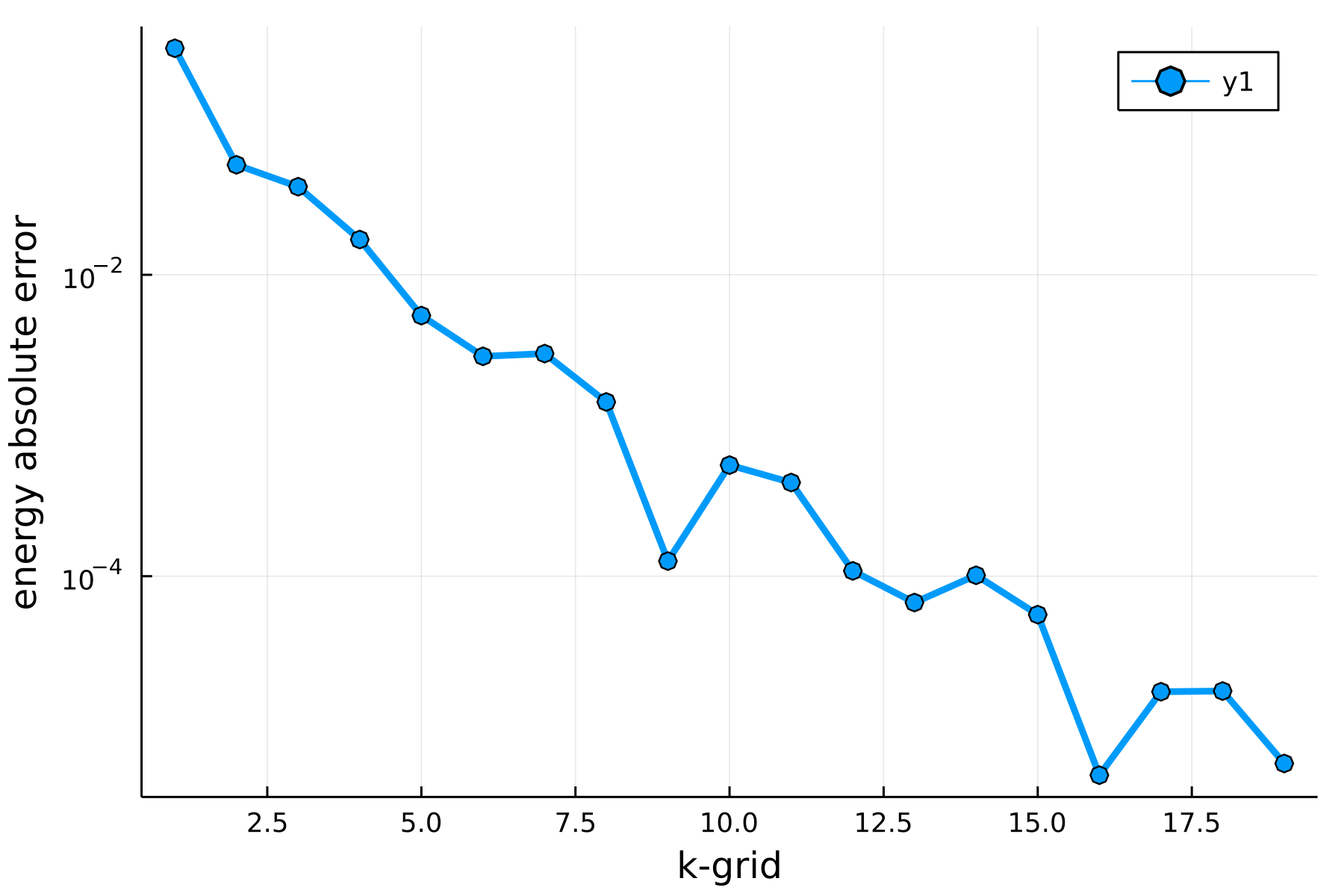
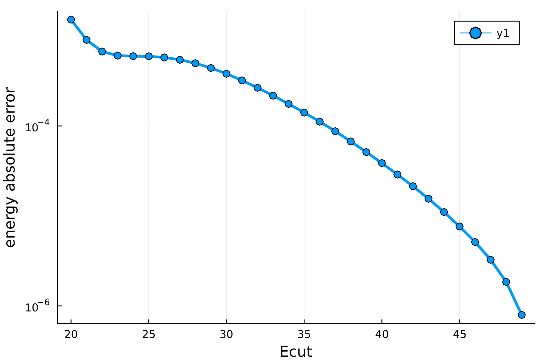
A more realistic example.¶

Repeating the above exercise for more realistic settings, namely …

In [7]:

tol   = 1e-4  # Tolerance to which we target to converge
nkpts = 1:20  # K-point range checked for convergence
Ecuts = 20:1:50;

…one obtains the following two plots for the convergence in kpoints and Ecut.