Pseudopotentials
In this example, we'll look at how to use various pseudopotential (PSP) formats in DFTK and discuss briefly the utility and importance of pseudopotentials.
Currently, DFTK supports norm-conserving (NC) PSPs in separable (Kleinman-Bylander) form. Two file formats can currently be read and used: analytical Hartwigsen-Goedecker-Hutter (HGH) PSPs and numeric Unified Pseudopotential Format (UPF) PSPs.
In brief, the pseudopotential approach replaces the all-electron atomic potential with an effective atomic potential. In this pseudopotential, tightly-bound core electrons are completely eliminated ("frozen") and chemically-active valence electron wavefunctions are replaced with smooth pseudo-wavefunctions whose Fourier representations decay quickly. Both these transformations aim at reducing the number of Fourier modes required to accurately represent the wavefunction of the system, greatly increasing computational efficiency.
Different PSP generation codes produce various file formats which contain the same general quantities required for pesudopotential evaluation. HGH PSPs are constructed from a fixed functional form based on Gaussians, and the files simply tablulate various coefficients fitted for a given element. UPF PSPs take a more flexible approach where the functional form used to generate the PSP is arbitrary, and the resulting functions are tabulated on a radial grid in the file. The UPF file format is documented on the Quantum Espresso Website.
In this example, we will compare the convergence of an analytical HGH PSP with a modern numeric norm-conserving PSP in UPF format from PseudoDojo. Then, we will compare the bandstructure at the converged parameters calculated using the two PSPs.
using DFTK
using Unitful
using Plots
using LazyArtifacts
import Main: @artifact_str # hide
Here, we will use a Perdew-Wang LDA PSP from PseudoDojo,
which is available in the
JuliaMolSim PseudoLibrary.
Directories in PseudoLibrary correspond to artifacts that you can load using artifact
strings which evaluate to a filepath on your local machine where the artifact has been
downloaded.
!!! note "Using the PseudoLibrary in your own calculations" Instructions for using the PseudoLibrary in your own calculations can be found in its documentation.
We load the HGH and UPF PSPs using load_psp, which determines the
file format using the file extension. The artifact string literal resolves to the
directory where the file is stored by the Artifacts system. So, if you have your own
pseudopotential files, you can just provide the path to them as well.
psp_hgh  = load_psp("hgh/lda/si-q4.hgh");
psp_upf  = load_psp(artifact"pd_nc_sr_lda_standard_0.4.1_upf/Si.upf");
┌ Warning: using Pkg instead of using LazyArtifacts is deprecated
│   caller = eval at boot.jl:385 [inlined]
└ @ Core ./boot.jl:385
 Downloading artifact: pd_nc_sr_lda_standard_0.4.1_upf
First, we'll take a look at the energy cutoff convergence of these two pseudopotentials. For both pseudos, a reference energy is calculated with a cutoff of 140 Hartree, and SCF calculations are run at increasing cutoffs until 1 meV / atom convergence is reached.
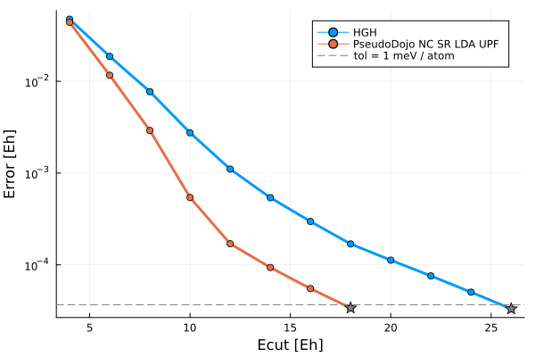
The converged cutoffs are 26 Ha and 18 Ha for the HGH and UPF pseudos respectively. We see that the HGH pseudopotential is much harder, i.e. it requires a higher energy cutoff, than the UPF PSP. In general, numeric pseudopotentials tend to be softer than analytical pseudos because of the flexibility of sampling arbitrary functions on a grid.
Next, to see that the different pseudopotentials give reasonbly similar results, we'll look at the bandstructures calculated using the HGH and UPF PSPs. Even though the convered cutoffs are higher, we perform these calculations with a cutoff of 12 Ha for both PSPs.
function run_bands(psp)
    a = 10.26  # Silicon lattice constant in Bohr
    lattice = a / 2 * [[0 1 1.];
                       [1 0 1.];
                       [1 1 0.]]
    Si = ElementPsp(:Si; psp)
    atoms     = [Si, Si]
    positions = [ones(3)/8, -ones(3)/8]

    # These are (as you saw above) completely unconverged parameters
    model = model_LDA(lattice, atoms, positions; temperature=1e-2)
    basis = PlaneWaveBasis(model; Ecut=12, kgrid=(4, 4, 4))

    scfres   = self_consistent_field(basis; tol=1e-4)
    bandplot = plot_bandstructure(compute_bands(scfres))
    (; scfres, bandplot)
end;
The SCF and bandstructure calculations can then be performed using the two PSPs, where we notice in particular the difference in total energies.
result_hgh = run_bands(psp_hgh)
result_hgh.scfres.energies
n     Energy            log10(ΔE)   log10(Δρ)   Diag   Δtime
---   ---------------   ---------   ---------   ----   ------
  1   -7.921038699554                   -0.69    5.8    453ms
  2   -7.925547576200       -2.35       -1.22    1.8    213ms
  3   -7.926172871958       -3.20       -2.42    2.9    574ms
  4   -7.926189237389       -4.79       -3.04    3.2    333ms
  5   -7.926189826841       -6.23       -4.08    2.5    531ms
Energy breakdown (in Ha):
    Kinetic             3.1589874
    AtomicLocal         -2.1423842
    AtomicNonlocal      1.6042681
    Ewald               -8.4004648
    PspCorrection       -0.2948928
    Hartree             0.5515432
    Xc                  -2.4000842
    Entropy             -0.0031626

    total               -7.926189826841
result_upf = run_bands(psp_upf)
result_upf.scfres.energies
n     Energy            log10(ΔE)   log10(Δρ)   Diag   Δtime
---   ---------------   ---------   ---------   ----   ------
  1   -8.515485098741                   -0.93    6.0    1.18s
  2   -8.518512950997       -2.52       -1.44    1.8    1.04s
  3   -8.518865400549       -3.45       -2.83    3.1    297ms
  4   -8.518884595936       -4.72       -3.20    4.4    368ms
  5   -8.518884691770       -7.02       -3.53    2.0    233ms
  6   -8.518884733365       -7.38       -4.59    1.5    213ms
Energy breakdown (in Ha):
    Kinetic             3.0954113
    AtomicLocal         -2.3650642
    AtomicNonlocal      1.3082420
    Ewald               -8.4004648
    PspCorrection       0.3951970
    Hartree             0.5521743
    Xc                  -3.1011608
    Entropy             -0.0032195

    total               -8.518884733365
But while total energies are not physical and thus allowed to differ, the bands (as an example for a physical quantity) are very similar for both pseudos:
plot(result_hgh.bandplot, result_upf.bandplot, titles=["HGH" "UPF"], size=(800, 400))